Example with IPD trial data

Introduction

This document runs a discrete event simulation model using simulated individual patient data (IPD) to show how the functions can be used to generate a model when IPD from a trial is available.

Packages and main options

library(WARDEN)
library(dplyr)
library(survival)
library(survminer)
library(kableExtra)
library(tidyr)
library(purrr)
library(flexsurv)

options(scipen = 999)
options(tibble.print_max = 50)

Model concept

All patients start in the progression-free state and may move to the progressed state. At any point in time they can die, depending on the risk of each disease stage. Patients may also experience a disease event which accelerates progression.

Generate dummy IPD trial data and fit survival models

The dummy IPD trial data was generated below from using the sim_adtte() function from the flexsurvPlus package. Parametric survival models are fit to the dummy OS and TTP IPD. We are using the flexsurv package to fit the parametric survival models.

#Generate dummy IPD
tte.df <- WARDEN::tte.df

#Change data frame to wide format
tte.df <- tte.df %>% select(-PARAM) %>% pivot_wider(names_from = PARAMCD, values_from = c(AVAL,CNSR)) 

#Derive Time to Progression Variable from OS and PFS
tte.df <- tte.df %>% mutate(
  AVAL_TTP = AVAL_PFS,
  CNSR_TTP = ifelse(AVAL_PFS == AVAL_OS & CNSR_PFS==0 & CNSR_OS==0,1,CNSR_PFS),
  Event_OS = 1-CNSR_OS,
  Event_PFS = 1-CNSR_PFS,
  Event_TTP = 1-CNSR_TTP
  )

#Add baseline characteristics (sex and age) to time to event data
IPD <- tte.df %>% mutate(
  SEX = rbinom(500,1,0.5),
  AGE = rnorm(500,60,8)
)

#Plot simulated OS and TTP curves

#Overall survival
km.est.OS <- survfit(Surv(AVAL_OS/365.25, Event_OS) ~ ARMCD, data = IPD) #KM curve

OS.fit <- flexsurvreg(formula = Surv(AVAL_OS/365.25, Event_OS) ~ ARMCD, data = IPD, dist = "Weibull") #Fit Weibull model to the OS data
OS.fit
#> Call:
#> flexsurvreg(formula = Surv(AVAL_OS/365.25, Event_OS) ~ ARMCD, 
#>     data = IPD, dist = "Weibull")
#> 
#> Estimates: 
#>         data mean  est     L95%    U95%    se      exp(est)  L95%    U95%  
#> shape       NA     1.1346  0.9764  1.3185  0.0870      NA        NA      NA
#> scale       NA     3.1523  2.5170  3.9479  0.3620      NA        NA      NA
#> ARMCDB  0.5000     0.3066  0.0183  0.5949  0.1471  1.3588    1.0185  1.8129
#> 
#> N = 500,  Events: 150,  Censored: 350
#> Total time at risk: 623.0253
#> Log-likelihood = -360.0964, df = 3
#> AIC = 726.1929

ggsurvplot(OS.fit, title="Overall survival",
           legend.labs = c("Reference","Intervention"),
           risk.table = TRUE)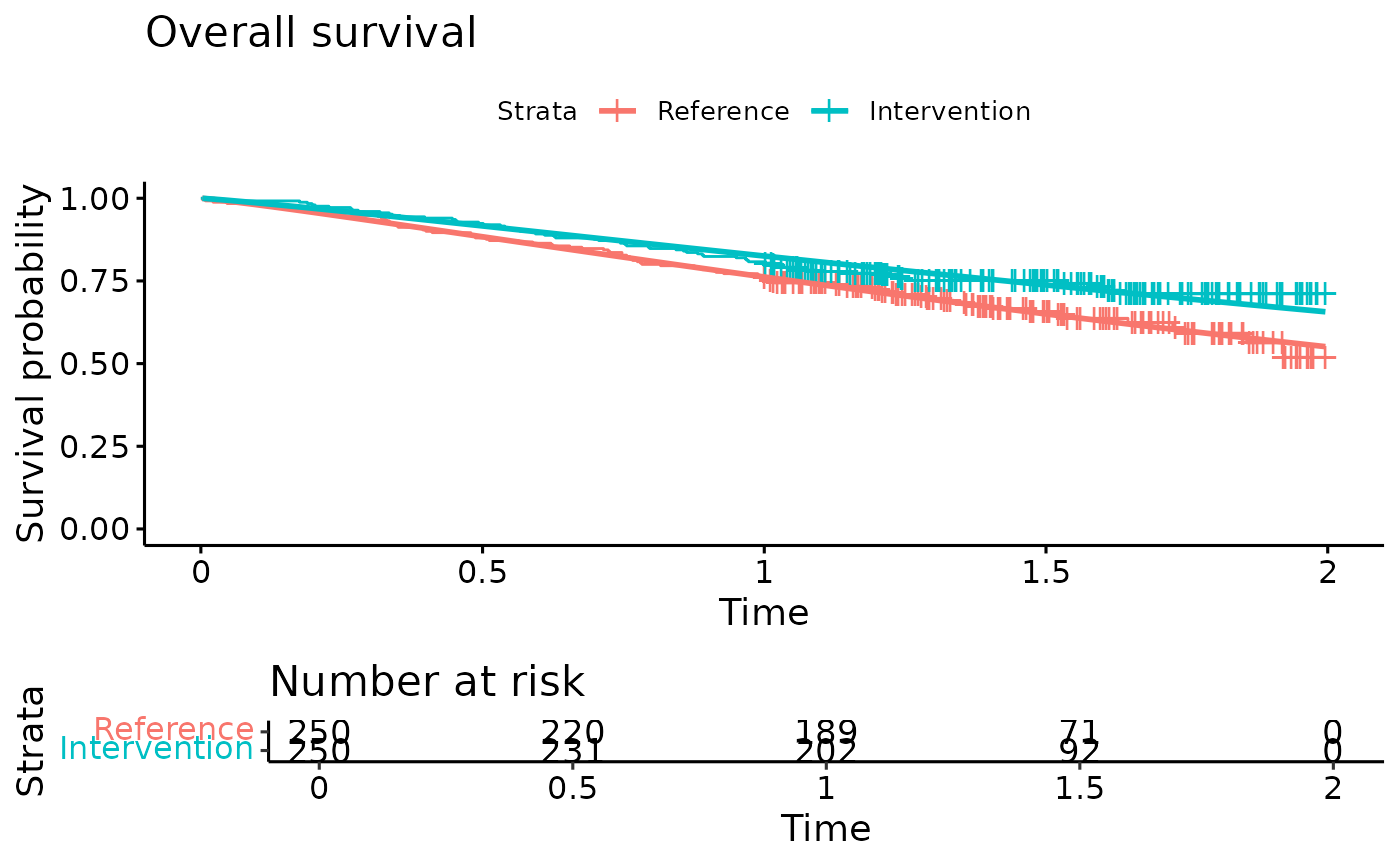


#Time to progression
km.est.TTP <- survfit(Surv(AVAL_TTP/365.25, Event_TTP) ~ ARMCD, data = IPD) #KM curve

TTP.fit <- flexsurvreg(formula = Surv(AVAL_TTP/365.25, Event_TTP) ~ ARMCD, data = IPD, dist = "Weibull") #Fit Weibull model to the TTP data
TTP.fit
#> Call:
#> flexsurvreg(formula = Surv(AVAL_TTP/365.25, Event_TTP) ~ ARMCD, 
#>     data = IPD, dist = "Weibull")
#> 
#> Estimates: 
#>         data mean  est     L95%    U95%    se      exp(est)  L95%    U95%  
#> shape       NA     1.3757  1.2590  1.5033  0.0622      NA        NA      NA
#> scale       NA     0.5865  0.5310  0.6478  0.0297      NA        NA      NA
#> ARMCDB  0.5000     1.0992  0.9277  1.2707  0.0875  3.0016    2.5286  3.5632
#> 
#> N = 500,  Events: 328,  Censored: 172
#> Total time at risk: 358.9897
#> Log-likelihood = -269.0387, df = 3
#> AIC = 544.0774

ggsurvplot(TTP.fit, title="Time to progression",
           legend.labs = c("Reference","Intervention"),
           risk.table = TRUE)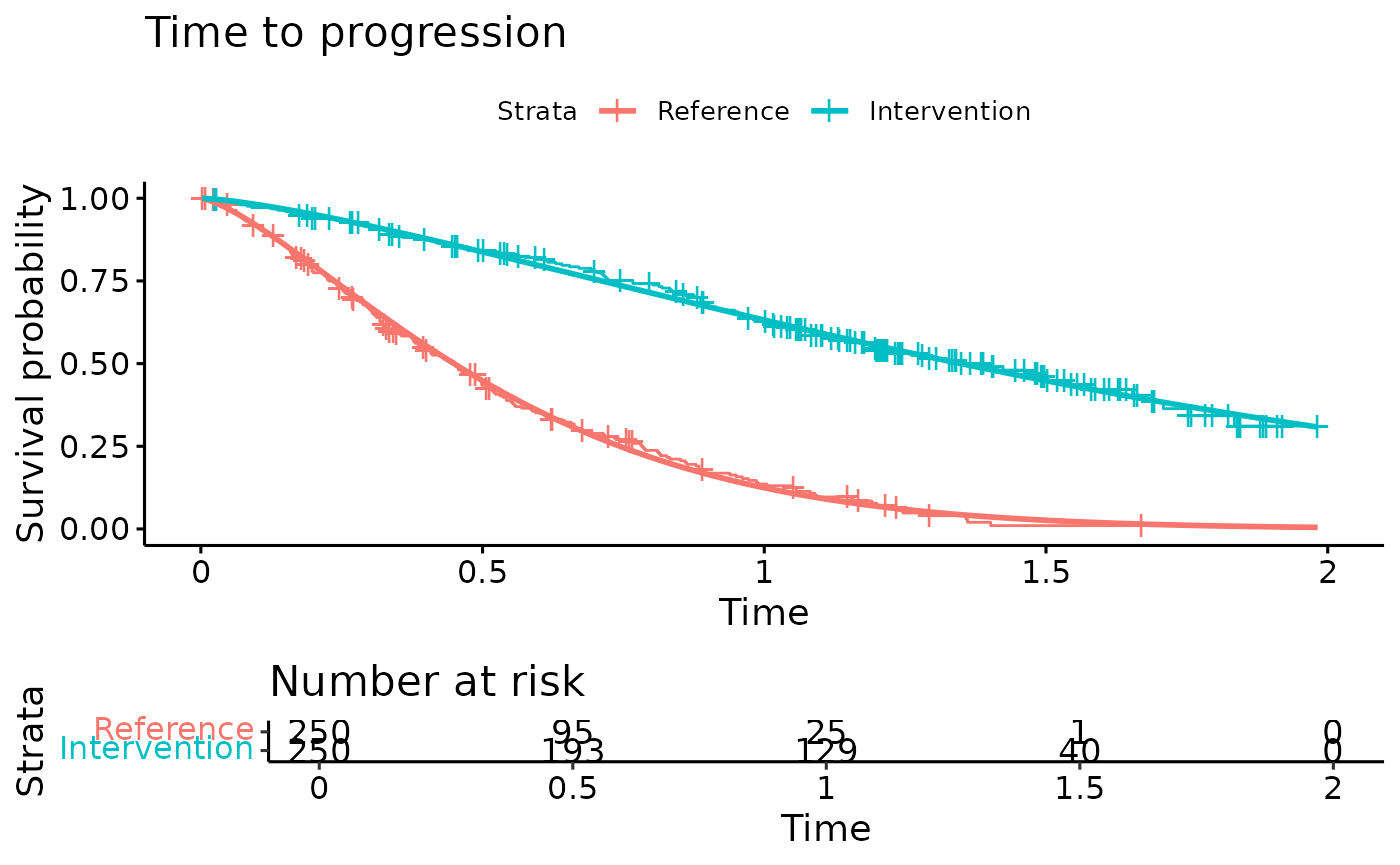

Define DES model inputs

Inputs and variables that will be used in the model are defined below. We can define inputs that are common to all patients (common_all_inputs) within a simulation, inputs that are unique to a patient independently of the treatment (e.g. natural death, defined in common_pt_inputs), and inputs that are unique to that patient and that treatment (unique_pt_inputs). Items can be included through the add_item() function, and can be used in subsequent items. All these inputs are generated before the events and the reaction to events are executed. Furthermore, the program first executes common_all_inputs, then common_pt_inputs and then unique_pt_inputs. So one could use the items generated in common_all_inputs in unique_pt_inputs.


#Define variables that do not change on any patient or intervention loop
common_all_inputs <- add_item( 
  #Parameters from the survival models
  OS.scale = as.numeric(OS.fit$coef[2]),
  OS.shape = as.numeric(OS.fit$coef[1]),
  OS.coef.int = as.numeric(OS.fit$coef[3]), #Intervention effect

  TTP.scale = as.numeric(TTP.fit$coef[2]),
  TTP.shape = as.numeric(TTP.fit$coef[1]),
  TTP.coef.int = as.numeric(TTP.fit$coef[3]), #Intervention effect
  
  #Utilities
  util.PFS = 0.6, #Utility while in progression-free state
  util.PPS = 0.4, #Utility while in progressed state
  disutil.PAE = -0.02, #One-off disutility of progression-accelerating event

  #Costs
  cost.drug.int = 85000, #Annual intervention cost
  cost.drug.ref = 29000, #Annual cost of reference treatment
  cost.admin.SC = 150, #Unit cost for each SC administration
  cost.admin.oral = 300, #One-off cost for oral administration
  cost.dm.PFS = 3000, #Annual disease-management cost in progression-free state
  cost.dm.PPS = 5000, #Annual disease-management cost in progressed state
  cost.ae.int = 2200, #Annual adverse event costs for intervention
  cost.ae.ref = 1400 #Annual adverse event costs for reference treatment
    )


#Define variables that do not change as we loop through interventions for a patient
common_pt_inputs <- add_item(
  #Patient baseline characteristics
  Sex = as.numeric(IPD[i,"SEX"]), #Record sex of individual patient. 0 = Female; 1 =Male
  BLAge = as.numeric(IPD[i,"AGE"]), #Record patient age at baseline
  
  #Draw time to non-disease related death from a conditional Gompertz distribution
  nat.death = rcond_gompertz(1,shape=if(Sex==1){0.102}else{0.115},
                               rate=if(Sex==1){0.000016}else{0.0000041},
                               lower_bound = BLAge) # Baseline Age in years
  )


#Define variables that change as we loop through treatments for each patient.
unique_pt_inputs <- add_item(
  fl.int  = 0, #Flag to determine if patient is on intervention. Initialized as 0, but will be changed to current arm in the Start event.
  fl.prog = 0, #Flag to determine if patient has progressed. All patients start progression-free
  fl.ontx = 1, #Flag to determine if patient is on treatment. All patients start on treatment
  fl.PAE = 0,  #Flag to determine if progression-accelerating event occurred
  pfs.time = NA, #Recording of time at progression
  q_default = ifelse(fl.prog == 0, util.PFS, util.PPS),
  q_default_inst = 0,
  c_default = ifelse(fl.prog == 0,cost.dm.PFS,cost.dm.PPS) + if(arm=="int"){(cost.drug.int + cost.admin.SC * 12 + cost.ae.int) * fl.ontx}else{cost.drug.ref + cost.ae.ref},
  c_default_inst = 0
)

Events

Add Initial Events

We define now the possible events that can occur for the intervention and reference arm respectively using the add_tte() function. Only patients in the intervention arm can have a treatment discontinuation, while patients in both arms can have a progression, progression-accelerating and death event. The seed argument is being used in the draw_tte() function which uses the i item to ensure that event times specific to each patient can be replicated and updated at later time points.

init_event_list <- 
  #Events applicable to intervention
  add_tte(arm=c("int","ref"),
          evts = c("Start",
                   "TxDisc",
                   "Progression",
                   "PAE",
                   "Death"),
               input={
    Start <- 0
    Progression <- draw_tte(1,'weibull',coef1=TTP.shape, coef2= TTP.scale + ifelse(arm=="int",TTP.coef.int,0),seed = as.numeric(paste0(1,i,simulation)))
    TxDisc <- Inf #Treatment discontinuation will occur at progression
    Death <- min(draw_tte(1,'weibull',coef1=OS.shape, coef2= OS.scale + ifelse(arm=="int",OS.coef.int,0), seed = as.numeric(paste0(42,i,simulation))), nat.death) #Death occurs at earliest of disease-related death or non-disease-related death
    PAE <- draw_tte(1,'exp',coef1=-log(1-ifelse(arm=="int",0.05,0.15))) #Occurrence of the progression-accelerating event has a 5% or 15% probability for the intervention arm
  })

Add Event Reactions

Reactions for each individual event are defined in the following using the add_reactevt() function. Patients in the intervention arm discontinue treatment at progression. Occurrence of the progression-accelerated event results in an earlier progression (if it has not occurred yet). Note the use of the seed argument in the draw_tte() function which ensures that the same seed is being used in the original and the updated draw of the time to progression.


evt_react_list <-
  add_reactevt(name_evt = "Start",
               input = {
                 fl.int = ifelse(arm=="int",1,0)
                 q_default = ifelse(fl.prog == 0, util.PFS, util.PPS)
                 c_default = ifelse(fl.prog == 0,cost.dm.PFS,cost.dm.PPS) + if(arm=="int"){(cost.drug.int + cost.admin.SC * 12 + cost.ae.int) * fl.ontx}else{cost.drug.ref + cost.ae.ref}
                 c_default_inst = cost.admin.oral
                                  
               }) %>%
  add_reactevt(name_evt = "TxDisc",
               input = {
                 q_default = ifelse(fl.prog == 0, util.PFS, util.PPS)
                 c_default = ifelse(fl.prog == 0,cost.dm.PFS,cost.dm.PPS) + if(arm=="int"){(cost.drug.int + cost.admin.SC * 12 + cost.ae.int) * fl.ontx}else{cost.drug.ref + cost.ae.ref}
                 fl.ontx = 0
               }) %>%
  add_reactevt(name_evt = "Progression",
               input = {
                 q_default = ifelse(fl.prog == 0, util.PFS, util.PPS)
                 c_default = ifelse(fl.prog == 0,cost.dm.PFS,cost.dm.PPS) + if(arm=="int"){(cost.drug.int + cost.admin.SC * 12 + cost.ae.int) * fl.ontx}else{cost.drug.ref + cost.ae.ref}
                 pfs.time=curtime
                 fl.prog= 1
                 if(arm=="int"){modify_event(c("TxDisc" = curtime))} #Trigger treatment discontinuation at progression
               }) %>%
  add_reactevt(name_evt = "Death",
               input = {
                 q_default = ifelse(fl.prog == 0, util.PFS, util.PPS)
                 c_default = ifelse(fl.prog == 0,cost.dm.PFS,cost.dm.PPS) + if(arm=="int"){(cost.drug.int + cost.admin.SC * 12 + cost.ae.int) * fl.ontx}else{cost.drug.ref + cost.ae.ref}
                 curtime = Inf
               }) %>%
  add_reactevt(name_evt = "PAE",
               input = {
                 fl.PAE = 1
                 q_default = ifelse(fl.prog == 0, util.PFS, util.PPS)
                 q_default_inst = disutil.PAE
                 c_default = ifelse(fl.prog == 0,cost.dm.PFS,cost.dm.PPS) + if(arm=="int"){(cost.drug.int + cost.admin.SC * 12 + cost.ae.int) * fl.ontx}else{cost.drug.ref + cost.ae.ref}
                 
                 if(fl.prog == 0){ #Event only accelerates progression if progression has not occurred yet
                 modify_event(c(
                   "Progression"=max(draw_tte(1,'weibull',coef1=TTP.shape, coef2= TTP.scale + TTP.coef.int*fl.int, beta_tx = 1.2, seed = as.numeric(paste0(1,i,simulation))),curtime))) #Occurrence of event accelerates progression by a factor of 1.2
                 }
               })

Costs and Utilities

Costs and utilities are introduced below.

Utilities


util_ongoing <- "q_default"

util_instant <- "q_default_inst"

Costs


cost_ongoing <- "c_default"

cost_instant <- "c_default_inst"

Model

Model Execution

The model is executed with the event reactions and inputs previously defined for each patient in the simulated data set.

#Logic is: per patient, per intervention, per event, react to that event.
results <- run_sim(  
  npats=as.numeric(nrow(IPD)),              # Simulating the number of patients for which we have IPD
  n_sim=1,                                  # We run all patients once (per treatment)
  psa_bool = FALSE,                         # No PSA for this example
  arm_list = c("int", "ref"),             
  common_all_inputs = common_all_inputs,    
  common_pt_inputs = common_pt_inputs,      
  unique_pt_inputs = unique_pt_inputs,      
  init_event_list = init_event_list,        
  evt_react_list = evt_react_list,          
  util_ongoing_list = util_ongoing,
  util_instant_list = util_instant,
  cost_ongoing_list = cost_ongoing,
  cost_instant_list = cost_instant,
  input_out = c("BLAge","Sex","nat.death","pfs.time")
)
#> Analysis number: 1
#> Simulation number: 1
#> Time to run simulation 1: 0.66s
#> Time to run analysis 1: 0.66s
#> Total time to run: 0.66s
#> Simulation finalized;

Post-processing of Model Outputs

Summary of Results

Once the model has been run, we can use the results and summarize them using the summary_results_det to print the results of the deterministic case. The individual patient data generated by the simulation is recorded in the psa_ipd object.


summary_results_det(results[[1]][[1]]) #will print the last simulation!
#>                              int        ref
#> costs                  261251.76   94361.19
#> dcosts                      0.00  166890.57
#> lys                         3.60       2.75
#> dlys                        0.00       0.85
#> qalys                       1.71       1.41
#> dqalys                      0.00       0.30
#> ICER                          NA  195784.55
#> ICUR                          NA  563768.08
#> INMB                          NA -152089.22
#> costs_undisc           286099.08  101986.36
#> dcosts_undisc               0.00  184112.72
#> lys_undisc                  3.99       2.97
#> dlys_undisc                 0.00       1.02
#> qalys_undisc                1.88       1.52
#> dqalys_undisc               0.00       0.35
#> ICER_undisc                   NA  180232.81
#> ICUR_undisc                   NA  518666.81
#> INMB_undisc                   NA -166364.07
#> BLAge                      59.66      59.66
#> dBLAge                      0.00       0.00
#> c_default              260951.76   94061.19
#> dc_default                  0.00  166890.57
#> c_default_inst            300.00     300.00
#> dc_default_inst             0.00       0.00
#> c_default_inst_undisc     300.00     300.00
#> dc_default_inst_undisc      0.00       0.00
#> c_default_undisc       285799.08  101686.36
#> dc_default_undisc           0.00  184112.72
#> nat.death                  24.33      24.33
#> dnat.death                  0.00       0.00
#> pfs.time                    1.61       0.58
#> dpfs.time                   0.00       1.03
#> q_default                   1.73       1.43
#> dq_default                  0.00       0.30
#> q_default_inst             -0.02      -0.02
#> dq_default_inst             0.00       0.00
#> q_default_inst_undisc      -0.02      -0.02
#> dq_default_inst_undisc      0.00       0.00
#> q_default_undisc            1.89       1.54
#> dq_default_undisc           0.00       0.36
#> Sex                         0.53       0.53
#> dSex                        0.00       0.00

psa_ipd <- bind_rows(map(results[[1]], "merged_df")) 

psa_ipd[1:10,] %>%
  kable() %>%
  kable_styling(bootstrap_options = c("striped", "hover", "condensed", "responsive"))

evtname	evttime	prevtime	pat_id	arm	total_lys	total_qalys	total_costs	total_costs_undisc	total_qalys_undisc	total_lys_undisc	lys	qalys	costs	lys_undisc	qalys_undisc	costs_undisc	BLAge	Sex	nat.death	pfs.time	c_default	c_default_inst	q_default	q_default_inst	c_default_undisc	q_default_undisc	c_default_inst_undisc	q_default_inst_undisc	nexttime	simulation	sensitivity
Start	0.0000000	0.000000	1	int	1.5055640	0.8841831	138811.88	141988.56	0.9040559	1.5400931	1.4288465	0.8573079	131753.8777	1.4598976	0.8759386	134610.5792	53.35829	0	30.07156	NA	131453.8777	300	0.8573079	0.0000000	134310.5792	0.8759386	300	0.00	1.4598976	1	1
PAE	1.4598976	0.000000	1	int	1.5055640	0.8841831	138811.88	141988.56	0.9040559	1.5400931	0.0767175	0.0268752	7058.0072	0.0801955	0.0281173	7377.9851	53.35829	0	30.07156	NA	7058.0072	0	0.0460305	-0.0191553	7377.9851	0.0481173	0	-0.02	1.5400931	1	1
Death	1.5400931	1.459898	1	int	1.5055640	0.8841831	138811.88	141988.56	0.9040559	1.5400931	0.0000000	0.0000000	0.0000	0.0000000	0.0000000	0.0000	53.35829	0	30.07156	NA	0.0000	0	0.0000000	0.0000000	0.0000	0.0000000	0	0.00	1.5400931	1	1
Start	0.0000000	0.000000	2	int	2.1750928	1.2858641	200408.54	207131.08	1.3288984	2.2481639	1.3675671	0.8205403	126116.1722	1.3959764	0.8375858	128729.8244	55.97126	1	36.09357	NA	125816.1722	300	0.8205403	0.0000000	128429.8244	0.8375858	300	0.00	1.3959764	1	1
PAE	1.3959764	0.000000	2	int	2.1750928	1.2858641	200408.54	207131.08	1.3288984	2.2481639	0.8075257	0.4653239	74292.3646	0.8521876	0.4913125	78401.2566	55.97126	1	36.09357	NA	74292.3646	0	0.4845154	-0.0191915	78401.2566	0.5113125	0	-0.02	2.2481639	1	1
Death	2.2481639	1.395976	2	int	2.1750928	1.2858641	200408.54	207131.08	1.3288984	2.2481639	0.0000000	0.0000000	0.0000	0.0000000	0.0000000	0.0000	55.97126	1	36.09357	NA	0.0000	0	0.0000000	0.0000000	0.0000	0.0000000	0	0.00	2.2481639	1	1
Start	0.0000000	0.000000	3	int	0.5544693	0.3326816	51311.17	51733.82	0.3354379	0.5590632	0.5544693	0.3326816	51311.1718	0.5590632	0.3354379	51733.8186	50.45087	1	25.36304	NA	51011.1718	300	0.3326816	0.0000000	51433.8186	0.3354379	300	0.00	0.5590632	1	1
Death	0.5590632	0.000000	3	int	0.5544693	0.3326816	51311.17	51733.82	0.3354379	0.5590632	0.0000000	0.0000000	0.0000	0.0000000	0.0000000	0.0000	50.45087	1	25.36304	NA	0.0000	0	0.0000000	0.0000000	0.0000	0.0000000	0	0.00	0.5590632	1	1
Start	0.0000000	0.000000	4	int	0.9496596	0.5503533	87668.68	88918.38	0.5579459	0.9632432	0.9431472	0.5658883	87069.5412	0.9565434	0.5739261	88301.9947	53.98621	0	37.38616	NA	86769.5412	300	0.5658883	0.0000000	88001.9947	0.5739261	300	0.00	0.9565434	1	1
PAE	0.9565434	0.000000	4	int	0.9496596	0.5503533	87668.68	88918.38	0.5579459	0.9632432	0.0065124	-0.0155350	599.1403	0.0066998	-0.0159801	616.3833	53.98621	0	37.38616	NA	599.1403	0	0.0039074	-0.0194424	616.3833	0.0040199	0	-0.02	0.9632432	1	1

We can also check what has been the absolute number of events per strategy.

arm	evtname	n
int	Death	500
int	Start	500
int	PAE	411
int	Progression	320
int	TxDisc	320
ref	Death	500
ref	Start	500
ref	Progression	441
ref	PAE	395

Plots

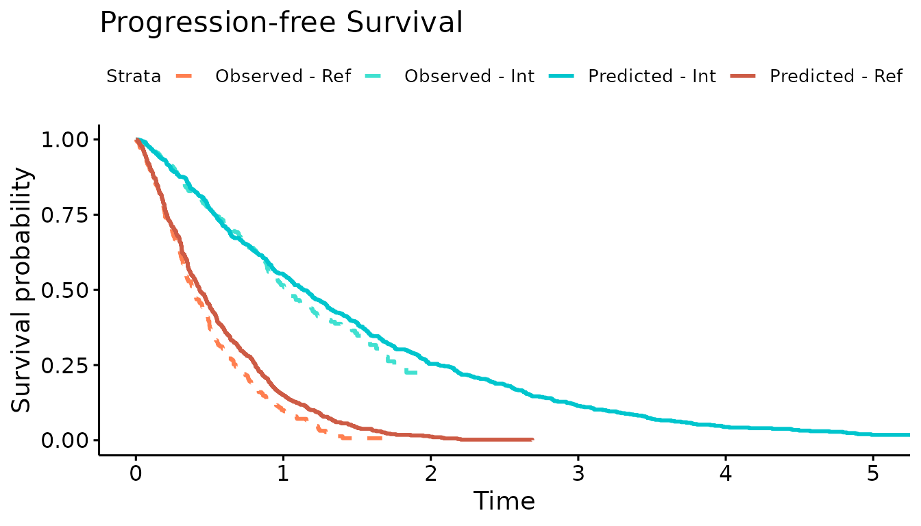
We now use the simulation output to plot the Kaplan-Meier curves of the simulated OS and PFS against the observed Kaplan-Meier curves. The simulated progression-free survival curve is lower than the observed due to the addition of the progression-accelerating event into the model.

#Overall survival
KM.death <- psa_ipd %>% filter(evtname=="Death") %>% mutate(Event = 1)

sim.km.OS <- survfit(Surv(evttime, Event) ~ arm, data = KM.death)

km.comb <- list(
  Observed = km.est.OS,
  Predicted = sim.km.OS
)

ggsurvplot(km.comb, combine = TRUE,
           title="Overall Survival",
           palette=c("coral","turquoise","turquoise3","coral3"),
           legend.labs=c("Observed - Ref","Observed - Int","Predicted - Int","Predicted - Ref"),
           linetype = c(2,2,1,1),
           xlim=c(0,10), break.time.by = 1, censor=FALSE)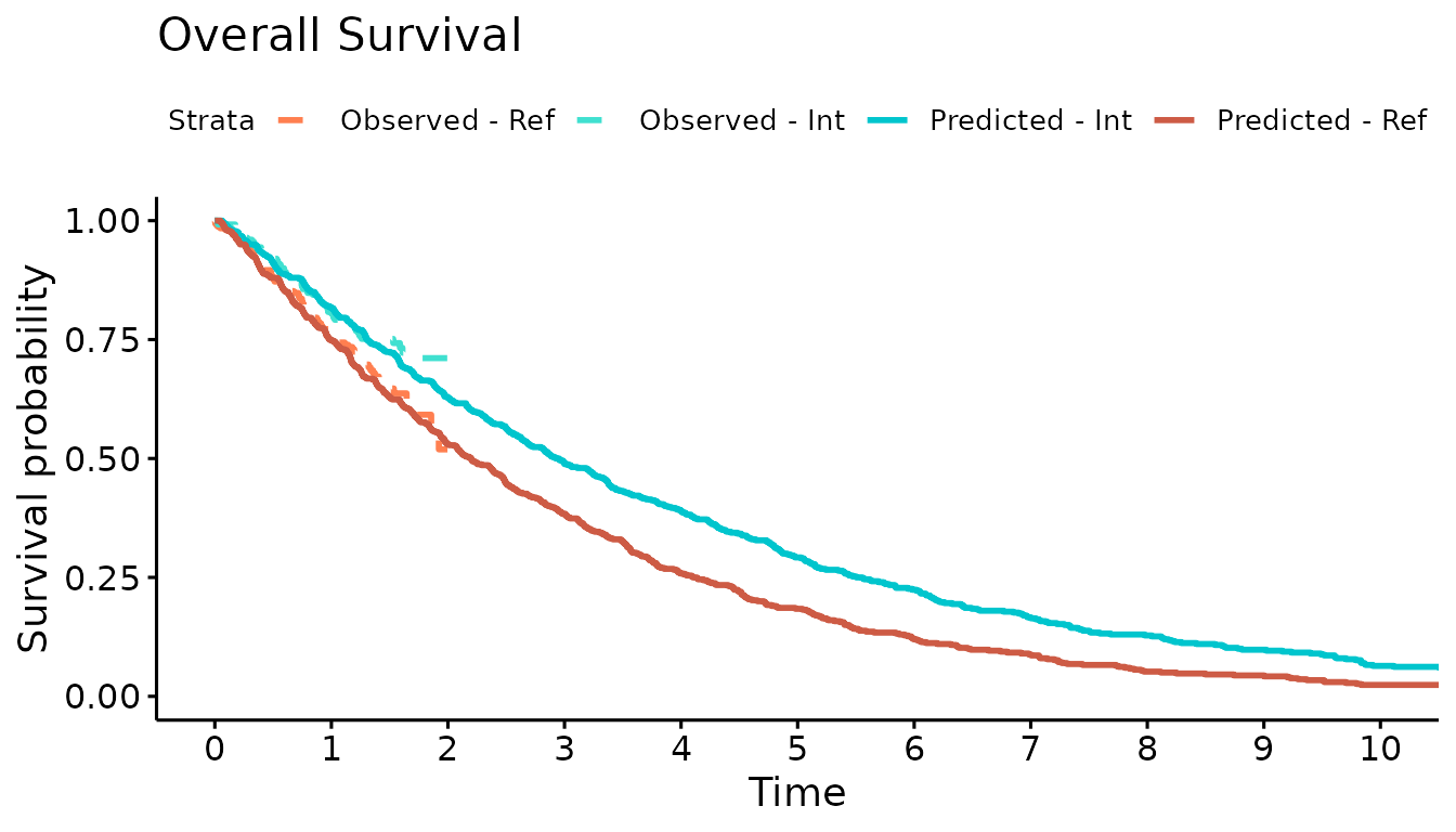


#Progression-free survival
km.est.PFS <- survfit(Surv(AVAL_PFS/365.25, Event_PFS) ~ ARMCD, data = IPD)
KM.PFS.DES <- psa_ipd %>% filter(evtname=="Death") %>% mutate(evttime = ifelse(is.na(pfs.time),evttime,pfs.time),
                                                          Event = 1)

sim.km.PFS <- survfit(Surv(evttime, Event) ~ arm, data = KM.PFS.DES)

km.comb <- list(Observed = km.est.PFS,
                Predicted = sim.km.PFS)

ggsurvplot(km.comb,combine = TRUE,
           title="Progression-free Survival",
           palette=c("coral","turquoise","turquoise3","coral3"),
           legend.labs=c("Observed - Ref","Observed - Int","Predicted - Int","Predicted - Ref"),
           linetype = c(2,2,1,1),
           xlim=c(0,5), break.time.by = 1, censor = FALSE)

Valerie Aponte Ribero and Javier Sanchez Alvarez

October 08, 2025