Example for a Resource Constrained Sick-Sicker-Dead model
Javier Sanchez Alvarez
July 24, 2026
Source:vignettes/articles/example_ssd_constrained.Rmd
example_ssd_constrained.RmdIntroduction
This document runs a discrete event simulation model in the context of a late oncology model to show how the functions can be used to generate a model in only a few steps. In this particular case, we document how to run a model with constrained resources.
Main options
library(WARDEN)

library(dplyr)
#>
#> Attaching package: 'dplyr'
#> The following objects are masked from 'package:stats':
#>
#>     filter, lag
#> The following objects are masked from 'package:base':
#>
#>     intersect, setdiff, setequal, union
library(ggplot2)
library(kableExtra)
#>
#> Attaching package: 'kableExtra'
#> The following object is masked from 'package:dplyr':
#>
#>     group_rows
library(purrr)General inputs with delayed execution
Compared to the standard sick-sicker-death model vignette, here nothing changes, except that now we add a resource which will be constrained (in a discrete manner, i.e., it accepts an integer amount of units and the resource can only be used unit-wise, like hospital beds, or doctors).
We should be careful about where we put the constrained resource, as
the level at which we set it up will determine its availability to
patients. Normally the intention is to have the resource being shared
within an arm by patients (and cloned across arms to make sure we
compare apples to apples), which means the resource should be allocated
in common_all_inputs (as those inputs will be cloned per
arm, so they will not be shared across arms unless explicitly declared
so using the specific constrained objects like
resource_discrete() or shared_input()). In our
case, we call the resource beds, and we use
resource_discrete() to set 650 beds to be shared. We also
keep track of the number of beds free for the purpose of seeing it in
the results.
For the sake of an example, we also create a shared input that we
will be updating as a counter of patients as they go through the
simulation, to showcase how inputs can be shared. Objects that are not
defined in resource_discrete() or
shared_inputs() will not be shared, and hard copies will be
made (unless the user introduces objects which are environments, in
which case by their own nature they will be modified by reference, so
they will be shared across analyses, simulations, arms, and patients, so
their use is not really recommended except for advanced R users).
Because of the way the constrained simulation works, it is very
important to pre-define any random numbers that will be used before the
simulation executes (normally at the unique_pt_inputs
level, though depends on the case, see below for an exception and the
early breast cancer model for the norm), and not to call the “r”
functions (rexp(), rpois()…) in the event
reactions. This is because the random state of the model will change as
it goes over the model, and the nature of the loop makes it so that the
random states can be mixed between patients between one simulation and
another if an event TTE is altered so its position in the queue changes
from one simulation to another. This is also very important if we want
to compare outcomes using constrained = FALSE and constrained = TRUE (as
in constrained = FALSE the random state is patient specific and can be
tracked, but in constrained is much harder to do so or would violate
CRAN norms).
#We don't need to use sensitivity_inputs here, so we don't add that object

#Put objects here that do not change on any patient or intervention loop
#We use add_item and add_item to showcase how the user can implement the inputs (either works, add_item is just faster)
common_all_inputs <-add_item(input = {
                      util.sick   <- 0.8
                      util.sicker <- 0.5
                      cost.sick   <- 3000
                      cost.sicker <- 7000
                      cost.int    <- 1000
                      coef_noint  <- log(0.2)
                      HR_int      <- 0.8
                      drc         <- 0.035 #different values than what's assumed by default
                      drq         <- 0.035
                      random_seed_sicker_i <- sample.int(100000,npats,replace = FALSE)
                      beds <- resource_discrete(650) #initialized with 650 beds
                      beds_free <- beds$n_free() #extract current n_free
                      shared_accumulator <- shared_input(0) #initialized at 0
                      value_accum <- shared_accumulator$value() #extract value
})


#Put objects here that do not change as we loop through treatments for a patient
common_pt_inputs <- add_item(death= max(0.0000001,rnorm(n=1, mean=12, sd=3)))

#Put objects here that change as we loop through treatments for each patient (e.g. events can affect fl.tx, but events do not affect nat.os.s)
unique_pt_inputs <- add_item(fl.sick = 1,
                             q_default = util.sick,
                             c_default = cost.sick + if(arm=="int"){cost.int}else{0},
                             had_to_queue = 0,
                             time_in_queue = NA,
                             beds_util = 0,
                             beds_n_using = 0L)
Events
Add Initial Events
Nothing changes here relative to the standard approach.
init_event_list <-
  add_tte(arm=c("noint","int"), evts = c("sick","sicker","death") ,input={
    sick <- 0
    sicker <- draw_tte(1,dist="exp", coef1=coef_noint, beta_tx = ifelse(arm=="int",HR_int,1), seed = random_seed_sicker_i[i]) #this way the value would be the same if it wasn't for the HR, effectively "cloning" patients luck

  })
Add Reaction to Those Events
We will assume that when the patients enter the sicker event, they attempt to use one of the beds. If they do so, everything goes as normal. If they fail to use one of the beds, the time to death is accelerated as they cannot get the right treatment.
The resource helpers seize() and release()
read i and curtime from the calling
environment automatically. seize(beds) returns
TRUE (acquired), FALSE (queued), or
NA (rejected when max_queue is set).
release(beds, resume_event = "sicker") frees the bed for
the current patient and, when a patient is queued, schedules their
"sicker" event automatically — eliminating the manual
if(was_using & queue_size > 0) new_event(...)
pattern.
Queue wait time and the queuing flag are now tracked in C++ inside
the resource object. beds$queue_wait_time_current() returns
NA if the patient never queued, 0 at the
moment they enter the queue, grows with elapsed time at each subsequent
event while waiting, and returns the total wait time once they acquire.
beds$had_to_queue() returns 0L or
1L and is a permanent per-patient flag.
evt_react_list <-
  add_reactevt(name_evt = "sick",
               input = {
                 value_accum   <- shared_incr(shared_accumulator, 1)
                 beds_free     <- beds$n_free()
                 beds_util     <- beds$utilization()
                 beds_n_using  <- beds$n_using()
               }) |>
  add_reactevt(name_evt = "sicker",
               input = {
                 acquired  <- seize(beds)
                 beds_free <- beds$n_free()
                 beds_util    <- beds$utilization()
                 beds_n_using <- beds$n_using()
                 if (!acquired) {
                   modify_event(c(death = max(curtime, get_event("death") * 0.8)))
                 }
                 had_to_queue  <- beds$had_to_queue()
                 q_default <- util.sicker
                 c_default <- cost.sicker + if(arm=="int"){cost.int}else{0}
                 fl.sick   <- 0
               }) |>
  add_reactevt(name_evt = "death",
               input = {
                 time_in_queue <- beds$queue_wait_time_current()
                 release(beds, resume_event = "sicker")
                 beds_free     <- beds$n_free()
                 beds_util     <- beds$utilization()
                 beds_n_using  <- beds$n_using()
                 q_default     <- 0
                 c_default     <- 0
                 curtime       <- Inf
})Model
Model Execution
The model is executed in exactly the same way as before, but we just
need to add constrained = TRUE to the arguments of
run_sim.
#Logic is: per patient, per intervention, per event, react to that event.
results <- run_sim(
  npats=1000,                               # number of patients to be simulated
  n_sim=1,                                  # number of simulations to run
  psa_bool = FALSE,                         # use PSA or not. If n_sim > 1 and psa_bool = FALSE, then difference in outcomes is due to sampling (number of pats simulated)
  arm_list = c("int", "noint"),             # intervention list
  common_all_inputs = common_all_inputs,    # inputs common that do not change within a simulation
  common_pt_inputs = common_pt_inputs,      # inputs that change within a simulation but are not affected by the intervention
  unique_pt_inputs = unique_pt_inputs,
  init_event_list = init_event_list,        # initial event list
  evt_react_list = evt_react_list,          # reaction of events
  util_ongoing_list = util_ongoing,
  cost_ongoing_list = cost_ongoing,
  constrained = TRUE,
  ipd = 1,
  input_out = c("beds_free","beds_util","beds_n_using","had_to_queue","time_in_queue","value_accum")
)
#> Analysis number: 1
#> Simulation number: 1
#> Time to run simulation 1: 1.05s
#> Time to run analysis 1: 1.05s
#> Total time to run: 1.05s
#> Simulation finalized;
Post-processing of model outputs
Summary of Results
summary_results_det(results[[1]][[1]]) #print first simulation
#>                        int    noint
#> costs             58978.88 50094.68
#> dcosts                0.00  8884.20
#> lys                   9.72     9.48
#> dlys                  0.00     0.24
#> qalys                 6.27     5.96
#> dqalys                0.00     0.31
#> ICER                    NA 37160.24
#> ICUR                    NA 28856.67
#> INMB                    NA  6509.47
#> costs_undisc      74324.03 62968.98
#> dcosts_undisc         0.00 11355.04
#> lys_undisc           11.99    11.63
#> dlys_undisc           0.00     0.36
#> qalys_undisc          7.62     7.20
#> dqalys_undisc         0.00     0.41
#> ICER_undisc             NA 31720.16
#> ICUR_undisc             NA 27387.61
#> INMB_undisc             NA  9375.22
#> beds_free           261.50   241.64
#> dbeds_free            0.00    19.87
#> beds_n_using        388.50   408.36
#> dbeds_n_using         0.00   -19.87
#> beds_util             0.60     0.63
#> dbeds_util            0.00    -0.03
#> c_default         58978.88 50094.68
#> dc_default            0.00  8884.20
#> c_default_undisc  74324.03 62968.98
#> dc_default_undisc     0.00 11355.04
#> had_to_queue          0.00     0.15
#> dhad_to_queue         0.00    -0.15
#> q_default             6.27     5.96
#> dq_default            0.00     0.31
#> q_default_undisc      7.62     7.20
#> dq_default_undisc     0.00     0.41
#> time_in_queue          NaN     0.65
#> dtime_in_queue         NaN      NaN
#> value_accum         500.50   500.50
#> dvalue_accum          0.00     0.00

psa_ipd <- bind_rows(map(results[[1]], "merged_df"))

psa_ipd[1:10,] |>
  kable() |>
kable_styling(bootstrap_options = c("striped", "hover", "condensed", "responsive"))| evtname | evttime | prevtime | pat_id | arm | total_lys | total_qalys | total_costs | total_costs_undisc | total_qalys_undisc | total_lys_undisc | lys | qalys | costs | lys_undisc | qalys_undisc | costs_undisc | beds_free | beds_util | beds_n_using | had_to_queue | time_in_queue | value_accum | c_default | q_default | c_default_undisc | q_default_undisc | nexttime | simulation | sensitivity |
|---|---|---|---|---|---|---|---|---|---|---|---|---|---|---|---|---|---|---|---|---|---|---|---|---|---|---|---|---|---|
| sick | 0.000 | 0.000 | 1 | int | 10.34 | 8.27 | 41358 | 51112 | 10.22 | 12.78 | 10.339 | 8.272 | 41358 | 12.778 | 10.222 | 51112 | 650 | 0.000 | 0 | 0 | NA | 1 | 41358 | 8.272 | 51112 | 10.222 | 12.778 | 1 | 1 |
| death | 12.778 | 0.000 | 1 | int | 10.34 | 8.27 | 41358 | 51112 | 10.22 | 12.78 | 0.000 | 0.000 | 0 | 0.000 | 0.000 | 0 | 313 | 0.518 | 337 | 0 | NA | 1 | 0 | 0.000 | 0 | 0.000 | 12.778 | 1 | 1 |
| sick | 0.000 | 0.000 | 2 | int | 7.75 | 4.14 | 58485 | 68551 | 4.78 | 9.02 | 0.887 | 0.710 | 3549 | 0.901 | 0.721 | 3604 | 650 | 0.000 | 0 | 0 | NA | 2 | 3549 | 0.710 | 3604 | 0.721 | 0.901 | 1 | 1 |
| sicker | 0.901 | 0.000 | 2 | int | 7.75 | 4.14 | 58485 | 68551 | 4.78 | 9.02 | 6.867 | 3.434 | 54937 | 8.118 | 4.059 | 64947 | 521 | 0.198 | 129 | 0 | NA | 2 | 54937 | 3.434 | 64947 | 4.059 | 9.019 | 1 | 1 |
| death | 9.019 | 0.901 | 2 | int | 7.75 | 4.14 | 58485 | 68551 | 4.78 | 9.02 | 0.000 | 0.000 | 0 | 0.000 | 0.000 | 0 | 32 | 0.951 | 618 | 0 | NA | 2 | 0 | 0.000 | 0 | 0.000 | 9.019 | 1 | 1 |
| sick | 0.000 | 0.000 | 3 | int | 10.94 | 5.57 | 86287 | 108582 | 6.96 | 13.73 | 0.317 | 0.253 | 1266 | 0.318 | 0.255 | 1273 | 650 | 0.000 | 0 | 0 | NA | 3 | 1266 | 0.253 | 1273 | 0.255 | 0.318 | 1 | 1 |
| sicker | 0.318 | 0.000 | 3 | int | 10.94 | 5.57 | 86287 | 108582 | 6.96 | 13.73 | 10.628 | 5.314 | 85020 | 13.414 | 6.707 | 107309 | 609 | 0.063 | 41 | 0 | NA | 3 | 85020 | 5.314 | 107309 | 6.707 | 13.732 | 1 | 1 |
| death | 13.732 | 0.318 | 3 | int | 10.94 | 5.57 | 86287 | 108582 | 6.96 | 13.73 | 0.000 | 0.000 | 0 | 0.000 | 0.000 | 0 | 405 | 0.377 | 245 | 0 | NA | 3 | 0 | 0.000 | 0 | 0.000 | 13.732 | 1 | 1 |
| sick | 0.000 | 0.000 | 4 | int | 8.61 | 5.24 | 56449 | 68546 | 6.10 | 10.22 | 3.116 | 2.493 | 12463 | 3.296 | 2.637 | 13183 | 650 | 0.000 | 0 | 0 | NA | 4 | 12463 | 2.493 | 13183 | 2.637 | 3.296 | 1 | 1 |
| sicker | 3.296 | 0.000 | 4 | int | 8.61 | 5.24 | 56449 | 68546 | 6.10 | 10.22 | 5.498 | 2.749 | 43986 | 6.920 | 3.460 | 55363 | 266 | 0.591 | 384 | 0 | NA | 4 | 43986 | 2.749 | 55363 | 3.460 | 10.216 | 1 | 1 |
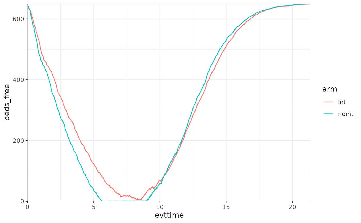
We can also check the evolution of the free beds over time per arm.
As it can be seen, 650 beds is just enough for the int arm
to handle all the requests, however in the noint arm there
are a few patients which must queue for some time. Note that the same
thing we do to see the number of free beds could be used to understand
the % of patients that were able to use a bed, etc. WARDEN is flexible
in that sense, one just needs to keep track of those numbers. For
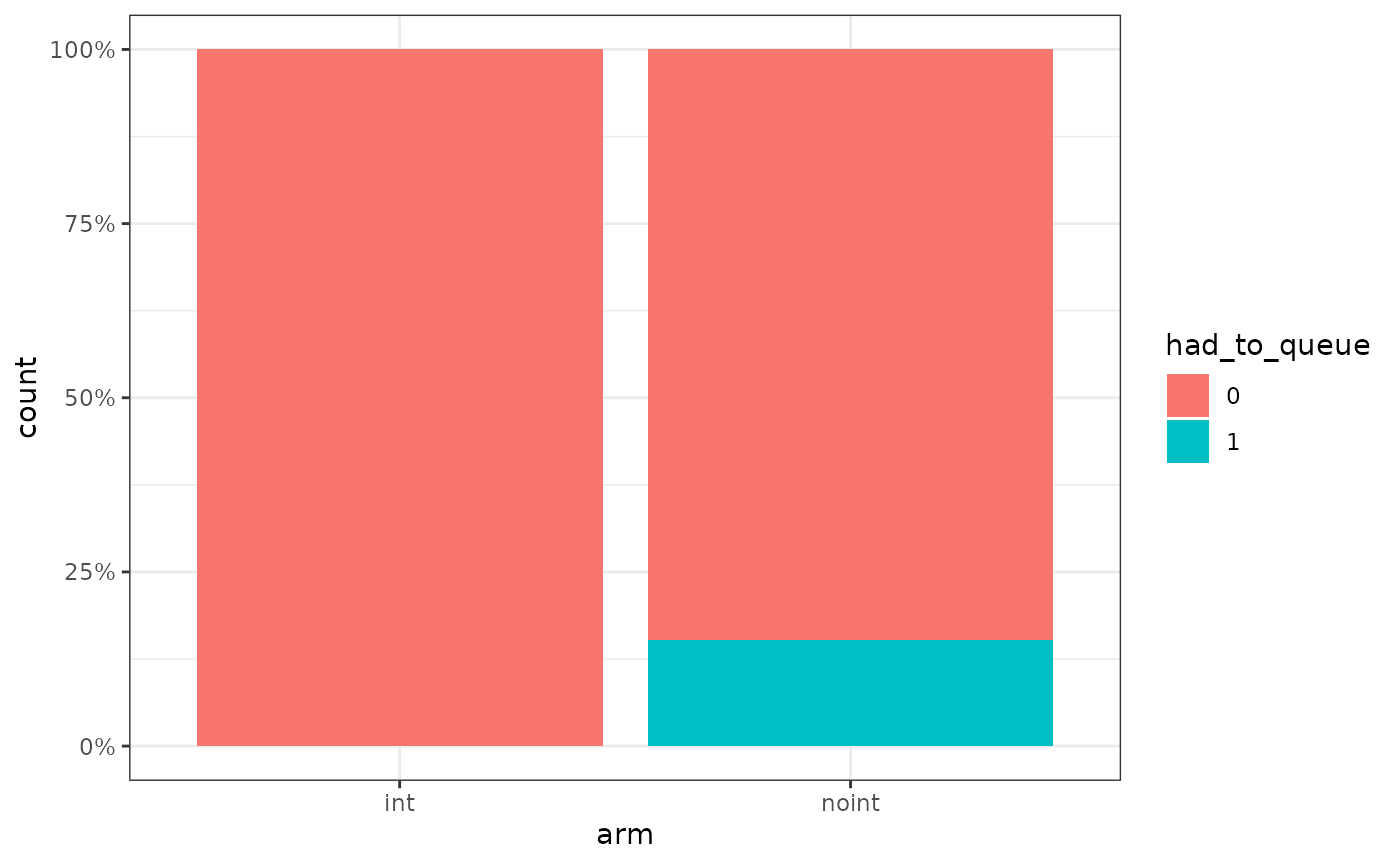
example, below we can see that around 15% of the noint
patients had to queue at a certain point. We can also track things like
queuing time, etc. In this case, for these 15% of patients, the average
queuing time was around 9 months.
#> Warning: Removed 1848 rows containing non-finite outside the scale range
#> (`stat_bin()`).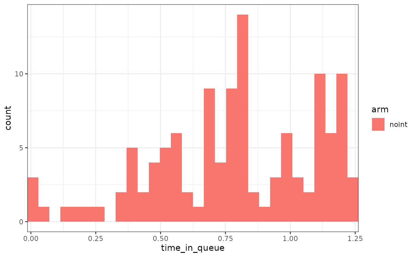
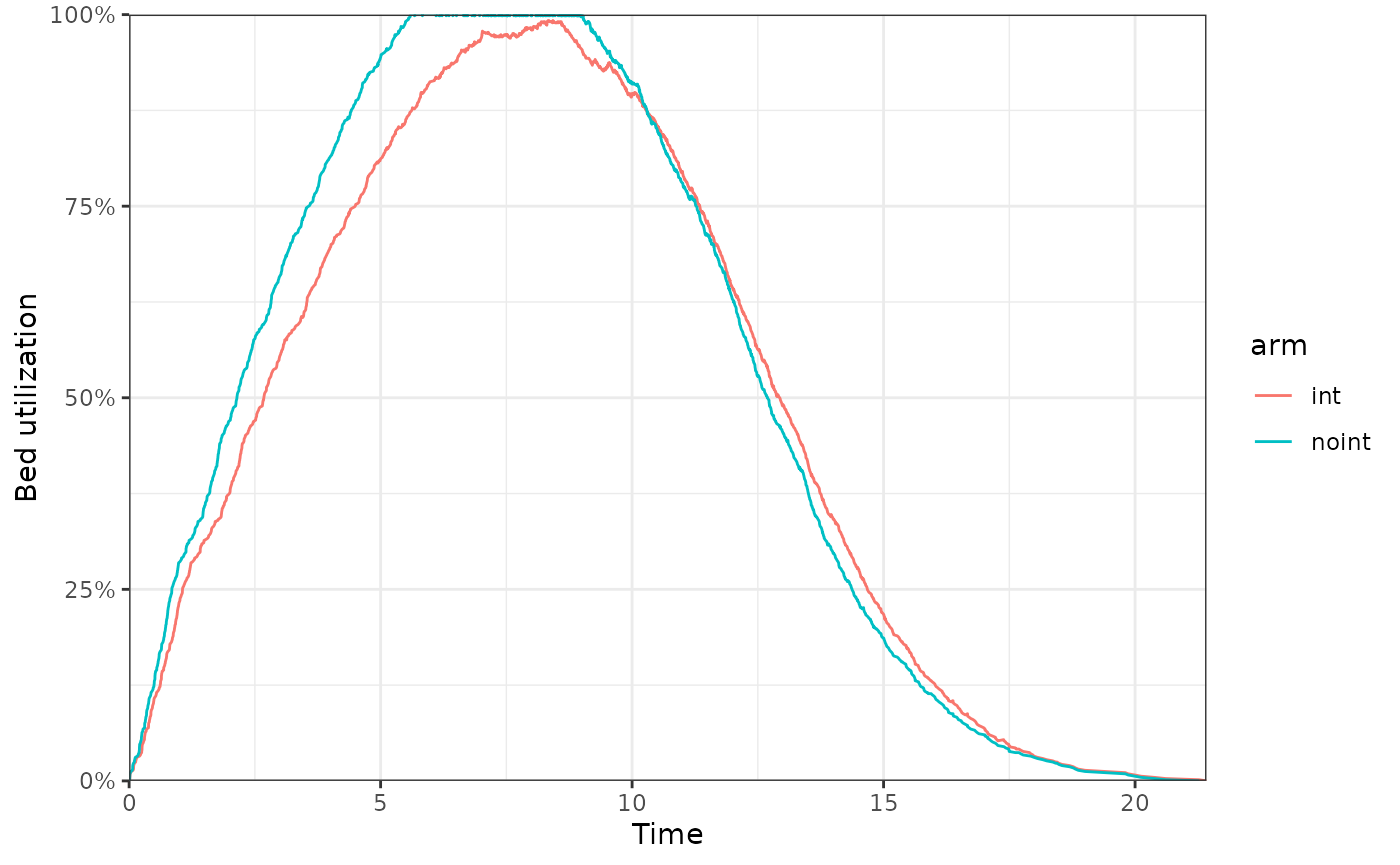
Resource statistics
Resource utilization (beds_util) and units in use
(beds_n_using) are tracked per event and exported via
input_out. We can plot bed utilization over time just like
beds_free:
The queue wait time (time_in_queue) and queuing flag
(had_to_queue) are computed inside the C++ resource and
read back in the reaction with
beds$queue_wait_time_current() and
beds$had_to_queue(). No manual bookkeeping is needed.
Sensitivity analysis
Run model with constrained = FALSE
It can be seen that with constrained = FALSE, the
results are equivalent to the SSD standard vignette. Furthermore, if the
model is run with constrained = TRUE but in such a way that the
constraint does not bind (e.g., with 1000+ beds) then the results are
also equivalent. If the model is run with
constrained = FALSE, then shared inputs and resources are
no longer shared. This allows to very quickly evaluate how the model
outputs change when resources are constrained vs. when they are not.
#Logic is: per patient, per intervention, per event, react to that event.
results <- run_sim(
  npats=1000,                               # number of patients to be simulated
  n_sim=1,                                  # number of simulations to run
  psa_bool = FALSE,                         # use PSA or not. If n_sim > 1 and psa_bool = FALSE, then difference in outcomes is due to sampling (number of pats simulated)
  arm_list = c("int", "noint"),             # intervention list
  common_all_inputs = common_all_inputs,    # inputs common that do not change within a simulation
  common_pt_inputs = common_pt_inputs,      # inputs that change within a simulation but are not affected by the intervention
  unique_pt_inputs = unique_pt_inputs,
  init_event_list = init_event_list,        # initial event list
  evt_react_list = evt_react_list,          # reaction of events
  util_ongoing_list = util_ongoing,
  cost_ongoing_list = cost_ongoing,
  constrained = FALSE,
  ipd = 1,
  input_out = c("beds_free","had_to_queue","time_in_queue")
)
#> Analysis number: 1
#> Simulation number: 1
#> Time to run simulation 1: 0.92s
#> Time to run analysis 1: 0.93s
#> Total time to run: 0.93s
#> Simulation finalized;

summary_results_det(results[[1]][[1]]) #print first simulation
#>                        int    noint
#> costs             58978.88 51768.23
#> dcosts                0.00  7210.66
#> lys                   9.72     9.72
#> dlys                  0.00     0.00
#> qalys                 6.27     6.08
#> dqalys                0.00     0.19
#> ICER                    NA      Inf
#> ICUR                    NA 38286.46
#> INMB                    NA  2206.06
#> costs_undisc      74324.03 65474.81
#> dcosts_undisc         0.00  8849.22
#> lys_undisc           11.99    11.99
#> dlys_undisc           0.00     0.00
#> qalys_undisc          7.62     7.38
#> dqalys_undisc         0.00     0.24
#> ICER_undisc             NA      Inf
#> ICUR_undisc             NA 37557.56
#> INMB_undisc             NA  2931.65
#> beds_free           650.00   650.00
#> dbeds_free            0.00     0.00
#> c_default         58978.88 51768.23
#> dc_default            0.00  7210.66
#> c_default_undisc  74324.03 65474.81
#> dc_default_undisc     0.00  8849.22
#> had_to_queue          0.00     0.00
#> dhad_to_queue         0.00     0.00
#> q_default             6.27     6.08
#> dq_default            0.00     0.19
#> q_default_undisc      7.62     7.38
#> dq_default_undisc     0.00     0.24
#> time_in_queue          NaN      NaN
#> dtime_in_queue         NaN      NaN
Run model constrained but unbinding
If the model is run with constrainted = TRUE but in such
a way that the constraint does not bind (e.g., with 1000+ beds) then the
results are also equivalent to constrained = FALSE.
common_all_inputs <-add_item(input = {
                      util.sick   <- 0.8
                      util.sicker <- 0.5
                      cost.sick   <- 3000
                      cost.sicker <- 7000
                      cost.int    <- 1000
                      coef_noint  <- log(0.2)
                      HR_int      <- 0.8
                      drc         <- 0.035 #different values than what's assumed by default
                      drq         <- 0.035
                      random_seed_sicker_i <- sample.int(100000,npats,replace = FALSE)
                      beds <- resource_discrete(1000)
                      beds_free <- beds$n_free()
                      shared_accumulator <- shared_input(0)
                      value_accum <- shared_accumulator$value()
})

#Logic is: per patient, per intervention, per event, react to that event.
results <- run_sim(
  npats=1000,                               # number of patients to be simulated
  n_sim=1,                                  # number of simulations to run
  psa_bool = FALSE,                         # use PSA or not. If n_sim > 1 and psa_bool = FALSE, then difference in outcomes is due to sampling (number of pats simulated)
  arm_list = c("int", "noint"),             # intervention list
  common_all_inputs = common_all_inputs,    # inputs common that do not change within a simulation
  common_pt_inputs = common_pt_inputs,      # inputs that change within a simulation but are not affected by the intervention
  unique_pt_inputs = unique_pt_inputs,
  init_event_list = init_event_list,        # initial event list
  evt_react_list = evt_react_list,          # reaction of events
  util_ongoing_list = util_ongoing,
  cost_ongoing_list = cost_ongoing,
  constrained = TRUE,
  ipd = 1,
  input_out = c("beds_free","had_to_queue","time_in_queue")
)
#> Analysis number: 1
#> Simulation number: 1
#> Time to run simulation 1: 1.12s
#> Time to run analysis 1: 1.13s
#> Total time to run: 1.13s
#> Simulation finalized;

summary_results_det(results[[1]][[1]]) #print first simulation
#>                        int    noint
#> costs             58978.88 51768.23
#> dcosts                0.00  7210.66
#> lys                   9.72     9.72
#> dlys                  0.00     0.00
#> qalys                 6.27     6.08
#> dqalys                0.00     0.19
#> ICER                    NA      Inf
#> ICUR                    NA 38286.46
#> INMB                    NA  2206.06
#> costs_undisc      74324.03 65474.81
#> dcosts_undisc         0.00  8849.22
#> lys_undisc           11.99    11.99
#> dlys_undisc           0.00     0.00
#> qalys_undisc          7.62     7.38
#> dqalys_undisc         0.00     0.24
#> ICER_undisc             NA      Inf
#> ICUR_undisc             NA 37557.56
#> INMB_undisc             NA  2931.65
#> beds_free           611.50   576.97
#> dbeds_free            0.00    34.53
#> c_default         58978.88 51768.23
#> dc_default            0.00  7210.66
#> c_default_undisc  74324.03 65474.81
#> dc_default_undisc     0.00  8849.22
#> had_to_queue          0.00     0.00
#> dhad_to_queue         0.00     0.00
#> q_default             6.27     6.08
#> dq_default            0.00     0.19
#> q_default_undisc      7.62     7.38
#> dq_default_undisc     0.00     0.24
#> time_in_queue          NaN      NaN
#> dtime_in_queue         NaN      NaN
Inputs
#Load some data
list_par <- list(parameter_name = list("util.sick","util.sicker","cost.sick","cost.sicker","cost.int","coef_noint","HR_int"),
                              base_value = list(0.8,0.5,3000,7000,1000,log(0.2),0.8),
                              DSA_min = list(0.6,0.3,1000,5000,800,log(0.1),0.5),
                              DSA_max = list(0.9,0.7,5000,9000,2000,log(0.4),0.9),
                              PSA_dist = list("rnorm","rbeta_mse","rgamma_mse","rgamma_mse","rgamma_mse","rnorm","rlnorm"),
                              a=list(0.8,0.5,3000,7000,1000,log(0.2),log(0.8)),
                              b=lapply(list(0.8,0.5,3000,7000,1000,log(0.2),log(0.8)), function(x) abs(x/5)),
                              scenario_1=list(0.6,0.3,1000,5000,800,log(0.1),0.5),
                              scenario_2=list(0.9,0.7,5000,9000,2000,log(0.4),0.9)
                              )

common_all_inputs <-
  input_block(base      = list_par[["base_value"]],
              psa       = pick_psa(list_par[["PSA_dist"]], rep(1, length(list_par[["PSA_dist"]])),
                                   list_par[["a"]], list_par[["b"]]),
              sens      = list_par,
              names_out = list_par[["parameter_name"]],
              dsa_names = c("DSA_min", "DSA_max")) |>
  add_item(input = {
    random_seed_sicker_i = sample(1:1000, 1000, replace = FALSE)
    beds <- resource_discrete(1000)
    beds_free <- beds$n_free()
    shared_accumulator <- shared_input(0)
    value_accum <- shared_accumulator$value()
  })
Model Execution
The model is executed as before, just adding
sensitivity_bool = TRUE. The n_sensitivity and
sensitivity_names arguments are auto-detected from the
input_block() metadata — no manual configuration
required.
results <- run_sim(
  npats=100,                               # number of patients to be simulated
  n_sim=1,                                  # number of simulations to run
  psa_bool = FALSE,                         # use PSA or not. If n_sim > 1 and psa_bool = FALSE, then difference in outcomes is due to sampling (number of pats simulated)
  arm_list = c("int", "noint"),             # intervention list
  common_all_inputs = common_all_inputs,    # inputs common that do not change within a simulation
  common_pt_inputs = common_pt_inputs,      # inputs that change within a simulation but are not affected by the intervention
  unique_pt_inputs = unique_pt_inputs,      # inputs that change within a simulation between interventions
  init_event_list = init_event_list,        # initial event list
  evt_react_list = evt_react_list,          # reaction of events
  util_ongoing_list = util_ongoing,
  cost_ongoing_list = cost_ongoing,
  sensitivity_bool = TRUE,
  constrained = TRUE,
  input_out = unlist(list_par[["parameter_name"]])
)
#> n_sensitivity auto-detected as 7 from input_block metadata
#> sensitivity_names auto-set to c("DSA_min", "DSA_max") from input_block metadata
#> Analysis number: 1
#> Simulation number: 1
#> Time to run simulation 1: 0.14s
#> Time to run analysis 1: 0.14s
#> Analysis number: 2
#> Simulation number: 1
#> Time to run simulation 1: 0.13s
#> Time to run analysis 2: 0.13s
#> Analysis number: 3
#> Simulation number: 1
#> Time to run simulation 1: 0.14s
#> Time to run analysis 3: 0.14s
#> Analysis number: 4
#> Simulation number: 1
#> Time to run simulation 1: 0.14s
#> Time to run analysis 4: 0.14s
#> Analysis number: 5
#> Simulation number: 1
#> Time to run simulation 1: 0.13s
#> Time to run analysis 5: 0.13s
#> Analysis number: 6
#> Simulation number: 1
#> Time to run simulation 1: 0.14s
#> Time to run analysis 6: 0.14s
#> Analysis number: 7
#> Simulation number: 1
#> Time to run simulation 1: 0.2s
#> Time to run analysis 7: 0.2s
#> Analysis number: 8
#> Simulation number: 1
#> Time to run simulation 1: 0.14s
#> Time to run analysis 8: 0.14s
#> Analysis number: 9
#> Simulation number: 1
#> Time to run simulation 1: 0.15s
#> Time to run analysis 9: 0.16s
#> Analysis number: 10
#> Simulation number: 1
#> Time to run simulation 1: 0.14s
#> Time to run analysis 10: 0.14s
#> Analysis number: 11
#> Simulation number: 1
#> Time to run simulation 1: 0.16s
#> Time to run analysis 11: 0.16s
#> Analysis number: 12
#> Simulation number: 1
#> Time to run simulation 1: 0.17s
#> Time to run analysis 12: 0.17s
#> Analysis number: 13
#> Simulation number: 1
#> Time to run simulation 1: 0.17s
#> Time to run analysis 13: 0.17s
#> Analysis number: 14
#> Simulation number: 1
#> Time to run simulation 1: 0.17s
#> Time to run analysis 14: 0.17s
#> Total time to run: 2.14s
#> Simulation finalized;
Check results
We briefly check below that indeed the engine has been changing the corresponding parameter value.
data_sensitivity <- bind_rows(map_depth(results,2, "merged_df"))

#Check mean value across iterations as PSA is off
data_sensitivity |> group_by(sensitivity) |> summarise_at(c("util.sick","util.sicker","cost.sick","cost.sicker","cost.int","coef_noint","HR_int"),mean)
#> # A tibble: 14 × 8
#>    sensitivity util.sick util.sicker cost.sick cost.sicker cost.int coef_noint
#>          <int>     <dbl>       <dbl>     <dbl>       <dbl>    <dbl>      <dbl>
#>  1           1       0.6         0.5      3000        7000     1000     -1.61
#>  2           2       0.8         0.3      3000        7000     1000     -1.61
#>  3           3       0.8         0.5      1000        7000     1000     -1.61
#>  4           4       0.8         0.5      3000        5000     1000     -1.61
#>  5           5       0.8         0.5      3000        7000      800     -1.61
#>  6           6       0.8         0.5      3000        7000     1000     -2.30
#>  7           7       0.8         0.5      3000        7000     1000     -1.61
#>  8           8       0.9         0.5      3000        7000     1000     -1.61
#>  9           9       0.8         0.7      3000        7000     1000     -1.61
#> 10          10       0.8         0.5      5000        7000     1000     -1.61
#> 11          11       0.8         0.5      3000        9000     1000     -1.61
#> 12          12       0.8         0.5      3000        7000     2000     -1.61
#> 13          13       0.8         0.5      3000        7000     1000     -0.916
#> 14          14       0.8         0.5      3000        7000     1000     -1.61
#> # ℹ 1 more variable: HR_int <dbl>
Model Execution, probabilistic DSA
The model is executed as before, just activating the psa_bool option
results <- run_sim(
  npats=100,
  n_sim=6,
  psa_bool = TRUE,
  arm_list = c("int", "noint"),
  common_all_inputs = common_all_inputs,
  common_pt_inputs = common_pt_inputs,
  unique_pt_inputs = unique_pt_inputs,
  init_event_list = init_event_list,
  evt_react_list = evt_react_list,
  util_ongoing_list = util_ongoing,
  cost_ongoing_list = cost_ongoing,
  sensitivity_bool = TRUE,
  constrained = TRUE,
  input_out = c(unlist(list_par[["parameter_name"]]), "beds_free")
)
#> n_sensitivity auto-detected as 7 from input_block metadata
#> sensitivity_names auto-set to c("DSA_min", "DSA_max") from input_block metadata
#> Analysis number: 1
#> Simulation number: 1
#> Time to run simulation 1: 0.15s
#> Simulation number: 2
#> Time to run simulation 2: 0.15s
#> Simulation number: 3
#> Time to run simulation 3: 0.15s
#> Simulation number: 4
#> Time to run simulation 4: 0.14s
#> Simulation number: 5
#> Time to run simulation 5: 0.16s
#> Simulation number: 6
#> Time to run simulation 6: 0.16s
#> Time to run analysis 1: 0.92s
#> Analysis number: 2
#> Simulation number: 1
#> Time to run simulation 1: 0.14s
#> Simulation number: 2
#> Time to run simulation 2: 0.16s
#> Simulation number: 3
#> Time to run simulation 3: 0.16s
#> Simulation number: 4
#> Time to run simulation 4: 0.14s
#> Simulation number: 5
#> Time to run simulation 5: 0.16s
#> Simulation number: 6
#> Time to run simulation 6: 0.16s
#> Time to run analysis 2: 0.93s
#> Analysis number: 3
#> Simulation number: 1
#> Time to run simulation 1: 0.14s
#> Simulation number: 2
#> Time to run simulation 2: 0.16s
#> Simulation number: 3
#> Time to run simulation 3: 0.16s
#> Simulation number: 4
#> Time to run simulation 4: 0.15s
#> Simulation number: 5
#> Time to run simulation 5: 0.15s
#> Simulation number: 6
#> Time to run simulation 6: 0.16s
#> Time to run analysis 3: 0.94s
#> Analysis number: 4
#> Simulation number: 1
#> Time to run simulation 1: 0.16s
#> Simulation number: 2
#> Time to run simulation 2: 0.14s
#> Simulation number: 3
#> Time to run simulation 3: 0.16s
#> Simulation number: 4
#> Time to run simulation 4: 0.17s
#> Simulation number: 5
#> Time to run simulation 5: 0.16s
#> Simulation number: 6
#> Time to run simulation 6: 0.2s
#> Time to run analysis 4: 1s
#> Analysis number: 5
#> Simulation number: 1
#> Time to run simulation 1: 0.18s
#> Simulation number: 2
#> Time to run simulation 2: 0.17s
#> Simulation number: 3
#> Time to run simulation 3: 0.15s
#> Simulation number: 4
#> Time to run simulation 4: 0.18s
#> Simulation number: 5
#> Time to run simulation 5: 0.16s
#> Simulation number: 6
#> Time to run simulation 6: 0.17s
#> Time to run analysis 5: 1.02s
#> Analysis number: 6
#> Simulation number: 1
#> Time to run simulation 1: 0.18s
#> Simulation number: 2
#> Time to run simulation 2: 0.15s
#> Simulation number: 3
#> Time to run simulation 3: 0.18s
#> Simulation number: 4
#> Time to run simulation 4: 0.17s
#> Simulation number: 5
#> Time to run simulation 5: 0.16s
#> Simulation number: 6
#> Time to run simulation 6: 0.18s
#> Time to run analysis 6: 1.01s
#> Analysis number: 7
#> Simulation number: 1
#> Time to run simulation 1: 0.16s
#> Simulation number: 2
#> Time to run simulation 2: 0.17s
#> Simulation number: 3
#> Time to run simulation 3: 0.18s
#> Simulation number: 4
#> Time to run simulation 4: 0.17s
#> Simulation number: 5
#> Time to run simulation 5: 0.16s
#> Simulation number: 6
#> Time to run simulation 6: 0.18s
#> Time to run analysis 7: 1.02s
#> Analysis number: 8
#> Simulation number: 1
#> Time to run simulation 1: 0.17s
#> Simulation number: 2
#> Time to run simulation 2: 0.16s
#> Simulation number: 3
#> Time to run simulation 3: 0.17s
#> Simulation number: 4
#> Time to run simulation 4: 0.18s
#> Simulation number: 5
#> Time to run simulation 5: 0.17s
#> Simulation number: 6
#> Time to run simulation 6: 0.16s
#> Time to run analysis 8: 1.01s
#> Analysis number: 9
#> Simulation number: 1
#> Time to run simulation 1: 0.17s
#> Simulation number: 2
#> Time to run simulation 2: 0.22s
#> Simulation number: 3
#> Time to run simulation 3: 0.16s
#> Simulation number: 4
#> Time to run simulation 4: 0.16s
#> Simulation number: 5
#> Time to run simulation 5: 0.17s
#> Simulation number: 6
#> Time to run simulation 6: 0.15s
#> Time to run analysis 9: 1.03s
#> Analysis number: 10
#> Simulation number: 1
#> Time to run simulation 1: 0.17s
#> Simulation number: 2
#> Time to run simulation 2: 0.17s
#> Simulation number: 3
#> Time to run simulation 3: 0.16s
#> Simulation number: 4
#> Time to run simulation 4: 0.19s
#> Simulation number: 5
#> Time to run simulation 5: 0.16s
#> Simulation number: 6
#> Time to run simulation 6: 0.17s
#> Time to run analysis 10: 1.02s
#> Analysis number: 11
#> Simulation number: 1
#> Time to run simulation 1: 0.18s
#> Simulation number: 2
#> Time to run simulation 2: 0.15s
#> Simulation number: 3
#> Time to run simulation 3: 0.17s
#> Simulation number: 4
#> Time to run simulation 4: 0.18s
#> Simulation number: 5
#> Time to run simulation 5: 0.16s
#> Simulation number: 6
#> Time to run simulation 6: 0.16s
#> Time to run analysis 11: 1.01s
#> Analysis number: 12
#> Simulation number: 1
#> Time to run simulation 1: 0.18s
#> Simulation number: 2
#> Time to run simulation 2: 0.17s
#> Simulation number: 3
#> Time to run simulation 3: 0.16s
#> Simulation number: 4
#> Time to run simulation 4: 0.18s
#> Simulation number: 5
#> Time to run simulation 5: 0.18s
#> Simulation number: 6
#> Time to run simulation 6: 0.2s
#> Time to run analysis 12: 1.07s
#> Analysis number: 13
#> Simulation number: 1
#> Time to run simulation 1: 0.16s
#> Simulation number: 2
#> Time to run simulation 2: 0.18s
#> Simulation number: 3
#> Time to run simulation 3: 0.17s
#> Simulation number: 4
#> Time to run simulation 4: 0.16s
#> Simulation number: 5
#> Time to run simulation 5: 0.18s
#> Simulation number: 6
#> Time to run simulation 6: 0.18s
#> Time to run analysis 13: 1.03s
#> Analysis number: 14
#> Simulation number: 1
#> Time to run simulation 1: 0.18s
#> Simulation number: 2
#> Time to run simulation 2: 0.17s
#> Simulation number: 3
#> Time to run simulation 3: 0.18s
#> Simulation number: 4
#> Time to run simulation 4: 0.48s
#> Simulation number: 5
#> Time to run simulation 5: 0.13s
#> Simulation number: 6
#> Time to run simulation 6: 0.14s
#> Time to run analysis 14: 1.29s
#> Total time to run: 14.31s
#> Simulation finalized;
Check results
We briefly check below that indeed the engine has been changing the
corresponding parameter value. As expected, beds_free is
only affected by the HR_int and coef_noint, as
those affect efficacy and therefore how beds are allocated.
data_sensitivity <- bind_rows(map_depth(results,2, "merged_df"))

#Check mean value across iterations as PSA is off
data_sensitivity |> group_by(sensitivity) |> summarise_at(c("util.sick","util.sicker","cost.sick","cost.sicker","cost.int","coef_noint","HR_int", "beds_free"),mean)
#> # A tibble: 14 × 9
#>    sensitivity util.sick util.sicker cost.sick cost.sicker cost.int coef_noint
#>          <int>     <dbl>       <dbl>     <dbl>       <dbl>    <dbl>      <dbl>
#>  1           1     0.6         0.580     3156.       7974.    1061.     -1.61
#>  2           2     0.722       0.3       3156.       7974.    1061.     -1.61
#>  3           3     0.722       0.580     1000        7974.    1061.     -1.61
#>  4           4     0.722       0.580     3156.       5000     1061.     -1.61
#>  5           5     0.722       0.580     3156.       7974.     800      -1.61
#>  6           6     0.725       0.579     3140.       7957.    1065.     -2.30
#>  7           7     0.722       0.580     3155.       7973.    1061.     -1.62
#>  8           8     0.9         0.580     3156.       7974.    1061.     -1.61
#>  9           9     0.722       0.7       3156.       7974.    1061.     -1.61
#> 10          10     0.722       0.580     5000        7974.    1061.     -1.61
#> 11          11     0.722       0.580     3156.       9000     1061.     -1.61
#> 12          12     0.722       0.580     3156.       7974.    2000      -1.61
#> 13          13     0.724       0.579     3145.       7962.    1066.     -0.916
#> 14          14     0.722       0.580     3156.       7973.    1062.     -1.62
#> # ℹ 2 more variables: HR_int <dbl>, beds_free <dbl>
Model Execution, Simple PSA
The model is executed as before, just activating the
psa_bool option and deactivating
sensitivity_bool.
common_all_inputs <-add_item(input = {
                      util.sick   <- 0.8
                      util.sicker <- 0.5
                      cost.sick   <- 3000
                      cost.sicker <- 7000
                      cost.int    <- 1000
                      coef_noint  <- log(0.2)
                      HR_int      <- 0.8
                      drc         <- 0.035 #different values than what's assumed by default
                      drq         <- 0.035
                      random_seed_sicker_i <- sample.int(100000,npats,replace = FALSE)
                      beds <- resource_discrete(65)
                      beds_free <- beds$n_free()
                      shared_accumulator <- shared_input(0)
                      value_accum <- shared_accumulator$value()

})


results <- run_sim(
  npats=100,
  n_sim=10,
  psa_bool = TRUE,
  arm_list = c("int", "noint"),
  common_all_inputs = common_all_inputs,
  common_pt_inputs = common_pt_inputs,
  unique_pt_inputs = unique_pt_inputs,
  init_event_list = init_event_list,
  evt_react_list = evt_react_list,
  util_ongoing_list = util_ongoing,
  cost_ongoing_list = cost_ongoing,
  sensitivity_bool = FALSE,
  constrained = TRUE,
  input_out = c(unlist(list_par[["parameter_name"]]), "beds_free")
)
#> Analysis number: 1
#> Simulation number: 1
#> Time to run simulation 1: 0.14s
#> Simulation number: 2
#> Time to run simulation 2: 0.15s
#> Simulation number: 3
#> Time to run simulation 3: 0.15s
#> Simulation number: 4
#> Time to run simulation 4: 0.14s
#> Simulation number: 5
#> Time to run simulation 5: 0.15s
#> Simulation number: 6
#> Time to run simulation 6: 0.14s
#> Simulation number: 7
#> Time to run simulation 7: 0.15s
#> Simulation number: 8
#> Time to run simulation 8: 0.15s
#> Simulation number: 9
#> Time to run simulation 9: 0.14s
#> Simulation number: 10
#> Time to run simulation 10: 0.15s
#> Time to run analysis 1: 1.47s
#> Total time to run: 1.47s
#> Simulation finalized;
Check results
We briefly check below that indeed the engine has been changing the
corresponding parameter values, and see how the free_beds
has been changing over time per simulation.
data_simulation <- bind_rows(map_depth(results,2, "merged_df"))

#Check mean value across iterations as PSA is off
data_simulation |> group_by(simulation) |> summarise_at(c("util.sick","util.sicker","cost.sick","cost.sicker","cost.int","coef_noint","HR_int", "beds_free"),mean)
#> # A tibble: 10 × 9
#>    simulation util.sick util.sicker cost.sick cost.sicker cost.int coef_noint
#>         <int>     <dbl>       <dbl>     <dbl>       <dbl>    <dbl>      <dbl>
#>  1          1       0.8         0.5      3000        7000     1000      -1.61
#>  2          2       0.8         0.5      3000        7000     1000      -1.61
#>  3          3       0.8         0.5      3000        7000     1000      -1.61
#>  4          4       0.8         0.5      3000        7000     1000      -1.61
#>  5          5       0.8         0.5      3000        7000     1000      -1.61
#>  6          6       0.8         0.5      3000        7000     1000      -1.61
#>  7          7       0.8         0.5      3000        7000     1000      -1.61
#>  8          8       0.8         0.5      3000        7000     1000      -1.61
#>  9          9       0.8         0.5      3000        7000     1000      -1.61
#> 10         10       0.8         0.5      3000        7000     1000      -1.61
#> # ℹ 2 more variables: HR_int <dbl>, beds_free <dbl>

ggplot(data_simulation,aes(x=evttime,y=beds_free, col = factor(simulation))) +
  facet_wrap(arm~.) +
  geom_line()+
  scale_y_continuous(expand = c(0, 0)) +
  scale_x_continuous(expand = c(0, 0)) +
  theme_bw()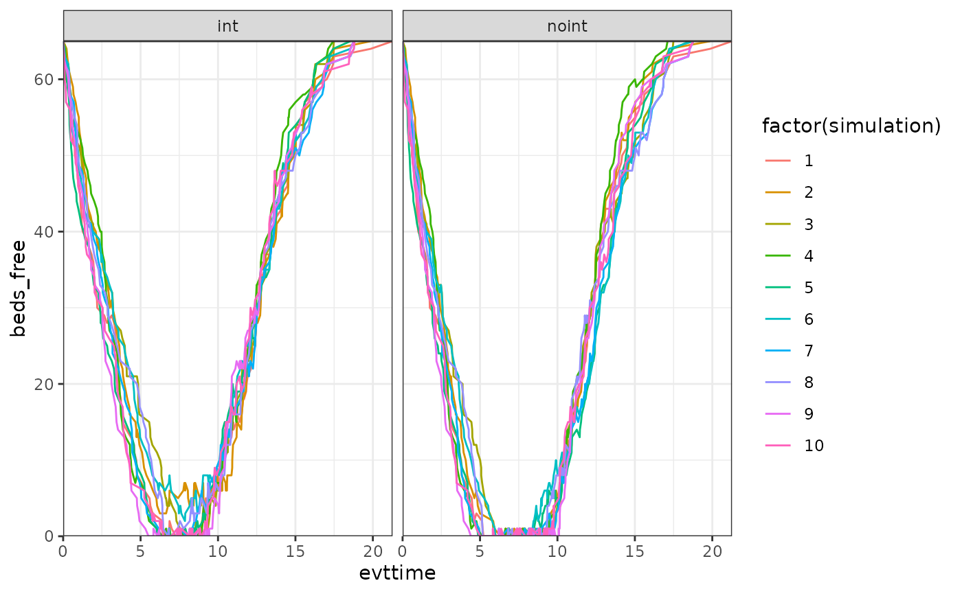
Multi-resource scheduling
When a patient needs multiple resources simultaneously (e.g., a bed
AND a specialist), seize_all() handles atomic acquisition
under "all_or_none" policy: the patient queues only for the
first unavailable resource, holding nothing else — deadlock-free by
design. Below is a complete model setup pattern using two resources.
# common_all_inputs — both resources initialized together
common_all_inputs_multi <- add_item(input = {
  util.sick   <- 0.8; util.sicker <- 0.5
  cost.sick   <- 3000; cost.sicker <- 7000; cost.int <- 1000
  coef_noint  <- log(0.2); HR_int <- 0.8; drc <- 0.035; drq <- 0.035
  random_seed_sicker_i <- sample.int(100000, npats, replace = FALSE)
  beds        <- resource_discrete(650)
  specialists <- resource_discrete(50)
  beds_free   <- beds$n_free()
  specialists_free   <- specialists$n_free()
})

unique_pt_inputs_multi <- add_item(input={
    if(arm=="int" & i == 1) specialists$add_resource(50) #add 50 specialists if arm == "int"
  }) |>
  add_item(
    fl.sick = 1,
    q_default = util.sick,
    c_default = cost.sick + if(arm == "int") cost.int else 0,
    had_to_queue = 0,
    time_in_queue = NA,
    specialists_free = 0L,
    beds_free = 0L
  )

evt_react_list_multi <-
  add_reactevt(name_evt = "sick", input = {
    beds_free        <- beds$n_free()
    specialists_free <- specialists$n_free()
    time_in_queue    <- NA
  }) |>
  add_reactevt(name_evt = "sicker", input = {
    # Patient needs BOTH a bed AND a specialist simultaneously.
    # seize_all with "all_or_none": queues only for the first unavailable resource.
    # With 650 beds vs 50 specialists, specialists saturate first, so patients
    # typically queue for specialists only, but can't use any.
    acquired <- seize_all(list(beds, specialists))
    beds_free        <- beds$n_free()
    specialists_free <- specialists$n_free()
    if (!acquired) {
      modify_event(c(death = max(curtime, get_event("death") * 0.8)))
    }
    # had_to_queue: 1 if queued for EITHER resource (check both)
    had_to_queue  <- max(beds$had_to_queue(), specialists$had_to_queue())
    # queue_wait_time_current: 0 at entry, grows while waiting, final wait on acquisition
    q_default <- util.sicker
    c_default <- cost.sicker + if(arm == "int") cost.int else 0
    fl.sick   <- 0
  }) |>
  add_reactevt(name_evt = "death", input = {
    time_in_queue <- specialists$queue_wait_time_current()
    # Release both resources; re-trigger the next patient queued for each
    release_all(list(beds, specialists), resume_event = "sicker")
    beds_free        <- beds$n_free()
    specialists_free <- specialists$n_free()
    q_default <- 0; c_default <- 0; curtime <- Inf
  })

results_multi <- run_sim(
  npats = 1000, n_sim = 1, psa_bool = FALSE,
  arm_list = c("int", "noint"),
  common_all_inputs = common_all_inputs_multi,
  common_pt_inputs = common_pt_inputs,
  unique_pt_inputs = unique_pt_inputs_multi,
  init_event_list = init_event_list,
  evt_react_list = evt_react_list_multi,
  util_ongoing_list = util_ongoing, cost_ongoing_list = cost_ongoing,
  constrained = TRUE, ipd = 1,
  input_out = c("beds_free","specialists_free","had_to_queue","time_in_queue")
)

psa_ipd <- bind_rows(map(results_multi[[1]], "merged_df"))
ggplot(psa_ipd) +
  geom_line(aes(x=evttime,y=beds_free, col = arm))+
  scale_y_continuous(expand = c(0, 0)) +
  scale_x_continuous(expand = c(0, 0)) +
  theme_bw()

ggplot(psa_ipd) +
  geom_line(aes(x=evttime,y=specialists_free, col = arm))+
  scale_y_continuous(expand = c(0, 0)) +
  scale_x_continuous(expand = c(0, 0)) +
  theme_bw()

ggplot(psa_ipd %>%
         filter(evtname=="death") %>%
         mutate(time_in_queue = ifelse(is.na(time_in_queue),0,time_in_queue)) %>%
         group_by(pat_id, arm) %>%
         summarise(time_in_queue = max(time_in_queue,na.rm=TRUE))
       ) +
  geom_histogram(aes(x=time_in_queue, fill = arm), alpha = 0.3, col = "white", position ="identity")+
  scale_y_continuous(expand = c(0, 0)) +
  scale_x_continuous(expand = c(0, 0)) +
  theme_bw()