Lin and Briggs (2025) Scottish CVD DES using WARDEN
Javier Sanchez Alvarez
July 24, 2026
Source:vignettes/articles/example_ScotCVD_LinBriggs.Rmd
example_ScotCVD_LinBriggs.RmdIntroduction
This document makes use of the code provided by Lin and Briggs (2025) which use R ad-hoc created functions to translate an existing Markov Scottish CVD model into a DES model. We showcase how the same model would be written with WARDEN.
Note that the model used is not resource constrained, so in WARDEN we
would use with the constrained = FALSE argument (which is
FALSE by default).
Main options
library(WARDEN)
library(flexsurv)
#> Loading required package: survival
library(dplyr)
#>
#> Attaching package: 'dplyr'
#> The following objects are masked from 'package:stats':
#>
#>     filter, lag
#> The following objects are masked from 'package:base':
#>
#>     intersect, setdiff, setequal, union
library(ggplot2)
library(kableExtra)
#>
#> Attaching package: 'kableExtra'
#> The following object is masked from 'package:dplyr':
#>
#>     group_rows
library(purrr)
library(tidyr)
if(!require(readxl)){
    install.packages("readxl")
    library(readxl)
}
#> Loading required package: readxl
if(!require(here)){
    install.packages("here")
    library(here)
}
#> Loading required package: here
#> here() starts at /home/runner/work/WARDEN/WARDEN

# Age in year (continuous)
# Normal distribution
list_age <- list(mean = 60, sd = 0, dist = "rnorm")

# Scottish Index of Multiple Deprivation (continuous, range: 0 to 100)
# Beta distribution
list_SIMD <- list(mean = 60.8, sd = 15, min = 0, max = 100, dist = "rbeta")

# % of diabetes (proportion, range: from 0 to 1)
# Bernoulli distribution for each patient
list_Diabetes <- list(prop = 0, label = c("yes", "no"))

# % of family history (proportion, range: from 0 to 1)
# Bernoulli distribution for each patient
list_FH <- list(prop = 0, label = c("yes", "no"))

# No. of cigarette per day (continuous)
# Gamma distribution
list_CPD <- list(mean = 20, sd = 0, dist = "rgamma")

# Systolic blood pressure (continuous)
# Normal distribution
list_SBP <- list(mean = 160, sd = 0, dist = "rnorm")

# Total cholesterol (continuous)
# Normal distribution
list_TC <- list(mean = 7, sd = 0, dist = "rnorm")

# High density cholesterol (continuous)
# Normal distribution
list_HDL <- list(mean = 1, sd = 0, dist = "rnorm")

# % of male (proportion, range: from 0 to 1)
# Bernoulli distribution for each patient
list_sex <- list(prop = 0.5, label = c("male", "female"))

tm <- 100 # maximum = 100
# time spline variables for cost models were reported up to t = 100
# (Lawson 2016. Appendix. Table A7 A8 A9 A10 A11 A12)

disc <- 0.035 # disc <-0 for undiscounted

# treatment effects on ldl and hdl
list_tx <- list(ldleffect = 0.26,
                hdleffect = 1.04,
                cost = 13,
                disu = 0.001)


sheet_names <- excel_sheets(here::here("data/CVDparameters.xlsx"))

list_coef <- lapply(seq_along(sheet_names),
                    function(x) {
  dt <- read_excel(here::here("data/CVDparameters.xlsx"), sheet = x, col_names = TRUE)
})

names(list_coef) <- sheet_names

list_coef2 <- list_coef

calib <- list(f1 = 0.96,
              multi_m = 0.99,
              multi_f = 1.05)

# Constant adjustment
j <- which(list_coef$first_event_coef_m$covariate == "constant")
list_coef$first_event_coef_m[j, -1] <- list_coef$first_event_coef_m[j, -1] *
  calib$multi_m
list_coef$first_event_coef_f[j, -1] <- list_coef$first_event_coef_f[j, -1] *
  calib$multi_f

# coefficient adjustment for TC and HDL for nonCVDdeath first event for male
j <- which(list_coef$first_event_coef_m$covariate %in% c("TC", "HDL"))
list_coef$first_event_coef_m[j, "first_event_nonCVD_death"] <- 0

# coefficient adjustment for TC CBVD and nonCVDdeath first events for female
j <- which(list_coef$first_event_coef_m$covariate %in% "TC")
list_coef$first_event_coef_f[j, c("first_event_nonfatal_CBVD", "first_event_nonCVD_death")] <- 0


list_coef <- lapply(list_coef, function(x) x |> keep(is.numeric) |> as.matrix())

list_u_norms <-
  list(
    u_norms_m = tibble(
      age = c("<25", "25-34", "35-44", "45-54", "55-64", "65-74", ">74"),
      age_min = c(0, 25, 35, 45, 55, 65, 75),
      age_max = c(25, 35, 45, 55, 65, 75, Inf),
      Index = c(0, seq(
        from = 25, to = 75, by = 10
      )),
      utility = c(0.831, 0.823, 0.820, 0.806, 0.801, 0.788, 0.774)
    ),
    u_norms_f = tibble(
      age = c("<25", "25-34", "35-44", "45-54", "55-64", "65-74", ">74"),
      age_min = c(0, 25, 35, 45, 55, 65, 75),
      age_max = c(25, 35, 45, 55, 65, 75, Inf),
      Index = c(0, seq(
        from = 25, to = 75, by = 10
      )),
      utility = c(0.809, 0.811, 0.802, 0.785, 0.787, 0.777, 0.721)
    )
  )

list_coef <- append(list_coef, list_u_norms)

rm(list_u_norms)


#RCS derived coefficients, directly from running the original code
nl_RCS <- list(
  nl_RCS_pre = list(
    male = list(
      knots = c(2, 7, 17),
      coef_a_1j = c(
        `(Intercept)` = -0.0355554000000008,
        C_ti1 = 0.0533331869047627,
        x2 = -0.0266666285714288,
        x3 = 0.00444444166666668
      ),
      coef_a_2j = c(
        `(Intercept)` = 2.25111027435915,
        C_ti1 = -0.926666325718771,
        x2 = 0.113333293706297,
        x3 = -0.002222220901321
      ),
      coef_a_3j = c(`(Intercept)` = -8.66666405454546,
                    C_ti1 = 0.999999754545455),
      r2_check = c(0.999999999999985, 0.999999999999987,
                   0.999999999999926)
    ),
    female = list(
      knots = c(2, 8, 17),
      coef_a_1j = c(
        `(Intercept)` = -0.0355553999999988,
        C_ti1 = 0.0533331869047611,
        x2 = -0.0266666285714284,
        x3 = 0.00444444166666666
      ),
      coef_a_2j = c(
        `(Intercept)` = 3.75704726107239,
        C_ti1 = -1.3688915683761,
        x2 = 0.151111334498837,
        x3 = -0.00296296891996898
      ),
      coef_a_3j = c(`(Intercept)` = -10.8,
                    C_ti1 = 1.2),
      r2_check = c(0.999999999999995, 0.999999999999996,
                   1)
    )
  ),
  nl_RCS_postCHD = list(
    male = list(
      knots = c(1, 6, 14),
      coef_a_1j = c(
        `(Intercept)` = -0.00591723333333363,
        C_ti1 = 0.0177515847883601,
        x2 = -0.0177515103174604,
        x3 = 0.00591716203703705
      ),
      coef_a_2j = c(
        `(Intercept)` = 2.07101078181822,
        C_ti1 = -1.02071181916788,
        x2 = 0.155325643795095,
        x3 = -0.00369823198653204
      ),
      coef_a_3j = c(`(Intercept)` = -8.07693209999999, C_ti1 = 1.15384662727273),
      r2_check = c(0.999999999999999, 0.999999999999992, 0.999999999999465)
    ),
    female = list(
      knots = c(1, 5, 12),
      coef_a_1j = c(
        `(Intercept)` = -0.00826453999999968,
        C_ti1 = 0.0247935047619046,
        x2 = -0.0247934285714285,
        x3 = 0.00826446666666666
      ),
      coef_a_2j = c(
        `(Intercept)` = 1.61511016623365,
        C_ti1 = -0.949231624530986,
        x2 = 0.170011662337658,
        x3 = -0.00472254343434329
      ),
      coef_a_3j = c(`(Intercept)` = -6.54546038181818,
                    C_ti1 = 1.09090950909091),
      r2_check = c(0.999999999999997, 0.999999999999993,
                   0.999999999999926)
    )
  ),
  nl_RCS_postCBVD = list(
    male = list(
      knots = c(1,
                5, 12),
      coef_a_1j = c(
        `(Intercept)` = -0.00826453999999968,
        C_ti1 = 0.0247935047619046,
        x2 = -0.0247934285714285,
        x3 = 0.00826446666666666
      ),
      coef_a_2j = c(
        `(Intercept)` = 1.61511016623365,
        C_ti1 = -0.949231624530986,
        x2 = 0.170011662337658,
        x3 = -0.00472254343434329
      ),
      coef_a_3j = c(`(Intercept)` = -6.54546038181818, C_ti1 = 1.09090950909091),
      r2_check = c(0.999999999999997, 0.999999999999993, 0.999999999999926)
    ),
    female = list(
      knots = c(1, 5, 12),
      coef_a_1j = c(
        `(Intercept)` = -0.00826453999999968,
        C_ti1 = 0.0247935047619046,
        x2 = -0.0247934285714285,
        x3 = 0.00826446666666666
      ),
      coef_a_2j = c(
        `(Intercept)` = 1.61511016623365,
        C_ti1 = -0.949231624530986,
        x2 = 0.170011662337658,
        x3 = -0.00472254343434329
      ),
      coef_a_3j = c(`(Intercept)` = -6.54546038181818,
                    C_ti1 = 1.09090950909091),
      r2_check = c(0.999999999999997, 0.999999999999993,
                   0.999999999999926)
    )
  )
)Conversion to WARDEN
Inputs
As with any model, we need to load inputs, set initial TTE, event
reactions, utilities/costs, etc. We’ll use the
input_block() function to have all inputs set-up at
once.
Though the model is a cohort one except for the SIMD variable, we assume here that we could use one with individual variation, so we define the parameters at the individual level instead of pre-loading them as a cohort (though we could do that as well). Since we do not have any uncertainty around the cohort parameters, we assume those are excluded from the PSA as in the original publication.
Normally, we would model each of the different events independently, i.e., we would allow the model to naturally choose and express the competitive risks (we would have an event for “nonfatal_CHD”, another for “nonfatal_CBVD”, etc), but for the sake of replication we will proceed as in the original paper, merging them into event 1 and event 2.
We create the time to event for the first event within the patient-arm level inputs.
We also create 3 ad-hoc functions to handle the restricted cube spline.
#helper functions for the restricted cube

rcs_du_v <-  function(du_all, du, t2, b5, b6, a0, a1, a2, a3){
  l_t <- length(t2)
  l_du <- length(du)

  # Polynomial term per time (length T)
  poly_t <- a3 * t2^3 + a2 * t2^2 + a1 * t2 + a0

  # Linear predictor matrix T × M
  # Each row t: du + b5*t + b6*poly(t)
  lp <- outer(t2, b5, "*") +            # B5 term: T×M
        outer(poly_t, b6, "*") +         # B6 * poly term: T×M
        matrix(du, l_t, l_du, byrow = TRUE)   # add du

  # Apply pnorm elementwise
  p <- pnorm(lp)

  # Weighted sum over DU_ALL (matrix multiply)
  drop(p %*% du_all)
}

disu_sec_vec <- function(time, DU_ALL, DU, B5, B6, nl_RCS_ch) {

  seg <- cut(
    time,
    breaks = c(-Inf, nl_RCS_ch$knots, Inf),
    labels = FALSE,
    right = FALSE
  )

  n <- length(time)
  a0 <- numeric(n); a1 <- a0; a2 <- a0; a3 <- a0

  s2 <- seg == 2
  if (any(s2)) {
    a0[s2] <- nl_RCS_ch[[2]][1]; a1[s2] <- nl_RCS_ch[[2]][2]
    a2[s2] <- nl_RCS_ch[[2]][3]; a3[s2] <- nl_RCS_ch[[2]][4]
  }

  s3 <- seg == 3
  if (any(s3)) {
    a0[s3] <- nl_RCS_ch[[3]][1]; a1[s3] <- nl_RCS_ch[[3]][2]
    a2[s3] <- nl_RCS_ch[[3]][3]; a3[s3] <- nl_RCS_ch[[3]][4]
  }

  rcs_du_v(
    t2    = time,
    du_all = DU_ALL,
    du    = DU,
    b5    = B5,
    b6    = B6,
    a0    = a0,
    a1    = a1,
    a2    = a2,
    a3    = a3
  )
}

rcs_cost_f <- function(time, nl_RCS_ch) {

  out <- numeric(length(time))
  knots <- nl_RCS_ch$knots

  i2 <- time >= knots[1] & time < knots[2]
  i3 <- time >= knots[2] & time < knots[3]
  i4 <- time >= knots[3]

  if (any(i2)) {
    t <- time[i2]; a <- nl_RCS_ch[[2]]
    out[i2] <- a[1] + t*(a[2] + t*(a[3] + t*a[4]))
  }

  if (any(i3)) {
    t <- time[i3]; a <- nl_RCS_ch[[3]]
    out[i3] <- a[1] + t*(a[2] + t*(a[3] + t*a[4]))
  }

  if (any(i4)) {
    t <- time[i4]; a <- nl_RCS_ch[[4]]
    out[i4] <- a[1] + a[2]*t
  }
  out
}
#reform parameters so it's clearer for model
l_CVD_inputs <- list(parameter_name = list(
                                      "first_event_nonfatal_CHD_m",
                                      "first_event_nonfatal_CBVD_m",
                                      "first_event_CVD_death_m",
                                      "first_event_nonCVD_death_m",
                                      "post_CHD_m",
                                      "post_CBVD_m",
                                      "first_event_nonfatal_CHD_f",
                                      "first_event_nonfatal_CBVD_f",
                                      "first_event_CVD_death_f",
                                      "first_event_nonCVD_death_f",
                                      "post_CHD_f",
                                      "post_CBVD_f"
                                      ),
                 base_value = list(
                    list_coef$first_event_coef_m[,1],
                    list_coef$first_event_coef_m[,2],
                    list_coef$first_event_coef_m[,3],
                    list_coef$first_event_coef_m[,4],
                    list_coef$post_event_coef_m[,1],
                    list_coef$post_event_coef_m[,2],
                    list_coef$first_event_coef_f[,1],
                    list_coef$first_event_coef_f[,2],
                    list_coef$first_event_coef_f[,3],
                    list_coef$first_event_coef_f[,4],
                    list_coef$post_event_coef_f[,1],
                    list_coef$post_event_coef_f[,2]
                   ),
                 PSA_dist = list("mvrnorm",
                                 "mvrnorm",
                                 "mvrnorm",
                                 "mvrnorm",
                                 "mvrnorm",
                                 "mvrnorm",
                                 "mvrnorm",
                                 "mvrnorm",
                                 "mvrnorm",
                                 "mvrnorm",
                                 "mvrnorm",
                                 "mvrnorm"
                                ),
                 a=list(
                    list_coef$first_event_coef_m[,1],
                    list_coef$first_event_coef_m[,2],
                    list_coef$first_event_coef_m[,3],
                    list_coef$first_event_coef_m[,4],
                    list_coef$post_event_coef_m[,1],
                    list_coef$post_event_coef_m[,2],
                    list_coef$first_event_coef_f[,1],
                    list_coef$first_event_coef_f[,2],
                    list_coef$first_event_coef_f[,3],
                    list_coef$first_event_coef_f[,4],
                    list_coef$post_event_coef_m[,1],
                    list_coef$post_event_coef_m[,2]
                   ),
                 b=list(
                    list_coef$cov_firstE_CHD_m,
                    list_coef$cov_firstE_CBVD_m,
                    list_coef$cov_fatal_CVD_m,
                    list_coef$cov_fatal_nonCVD_m,
                    list_coef$cov_surv_postCHD_m,
                    list_coef$cov_surv_postCBVD_m,
                    list_coef$cov_firstE_CHD_f,
                    list_coef$cov_firstE_CBVD_f,
                    list_coef$cov_fatal_CVD_f,
                    list_coef$cov_fatal_nonCVD_f,
                    list_coef$cov_surv_postCHD_f,
                    list_coef$cov_surv_postCBVD_f
                   ),
                 n=list(1,1,1,1,1,1,1,1,1,1,1,1),
                 psa_indicators = list(1,1,1,1,1,1,1,1,1,1,1,1)
                 )


common_all_inputs <-
  add_item(input = {
    drc       <- disc
    drq       <- disc
    ldleffect <- 0.26
    hdleffect <- 1.04
    cost_tx   <- 13
    cost      <- 0
    disu      <- 0.001
    f1        <- 0.96
    multi_m   <- 0.99
    multi_f   <- 1.05
    time_horizon <- tm
    age_v      <- rnorm(npats, list_age$mean, list_age$sd)
    SIMD_v     <- rbeta_mse(npats, list_SIMD$mean/100, list_SIMD$sd/100)
    Diabetes_v <- rbinom(npats, 1, list_Diabetes$prop)
    FH_v       <- rbinom(npats, 1, list_FH$prop)
    CPD_v      <- rgamma_mse(npats, list_CPD$mean, list_CPD$sd)
    SBP_v      <- rnorm(npats, list_SBP$mean, list_SBP$sd)
    TC_v       <- rnorm(npats, list_TC$mean, list_TC$sd)
    HDL_v      <- rnorm(npats, list_HDL$mean, list_HDL$sd)
    sex_v      <- rbinom(npats, 1, list_sex$prop)
    status_v   <- rep(0, npats)
  }) |>
  input_block(base            = l_CVD_inputs[["base_value"]],
              psa             = pick_psa(l_CVD_inputs[["PSA_dist"]],
                                         l_CVD_inputs[["n"]],
                                         l_CVD_inputs[["a"]],
                                         l_CVD_inputs[["b"]]),
              sens            = NULL,
              names_out       = l_CVD_inputs[["parameter_name"]],
              psa_indicators  = l_CVD_inputs[["psa_indicators"]],
              sens_indicators = rep(0L, 12),
              indicator_sens_binary = TRUE) |>
  add_item(input = {
    odd_seq <- seq(1, 10, 2)
    even_seq <- seq(2, 10, 2)
    q_total  <- 0
  })


common_pt_inputs <- add_item(input={
    sex <- sex_v[i]
    bs_age <- age_v[i]
    age <- bs_age
    SIMD <- SIMD_v[i] * 100
    Diabetes <- Diabetes_v[i]
    FH <- FH_v[i]
    CPD <- CPD_v[i]
    SBP <- SBP_v[i]
    status <- status_v[i]
    u_norms <- if(sex == 1){list_coef$u_norms_m}else{list_coef$u_norms_f}
    v_du <- if(sex == 1){list_coef$coef_u_m}else{list_coef$coef_u_f}
    v_du <- c(v_du,0) #append 0 for time horizon case
    second_event_du_coef <- if(sex == 1){list_coef$second_event_coef_m}else{list_coef$second_event_coef_f}
    coef_c1 <- if(sex == 1){list_coef$coef_c1_m}else{list_coef$coef_c1_f}
    coef_c1_pre <- coef_c1[,c(1,2,5,6)]
    coef_c1_post <- coef_c1[,c(3,4)]
    coef_c2 <- if(sex == 1){list_coef$coef_c2_m}else{list_coef$coef_c2_f}
    post_CHD <- if(sex == 1){post_CHD_m}else{post_CHD_f}
    post_CBVD <- if(sex == 1){post_CBVD_m}else{post_CBVD_f}
    rnd_v_1 <- runif(4)
    rnd_v_2 <- runif(2)
})

unique_pt_inputs <- add_item(input = {
    treatment <- as.numeric(arm == "int")
    TC  <- TC_v[i] - (TC_v[i] - HDL_v[i]) * treatment * ldleffect
    HDL <- HDL_v[i] * hdleffect ^ treatment

    m_pat_ch <- matrix(c(age, SIMD, Diabetes, FH, CPD, SBP, TC, HDL, 1), ncol = 9)
    first_event_nonfatal_CHD <- if(sex == 1){first_event_nonfatal_CHD_m}else{first_event_nonfatal_CHD_f}
    lp_first_event_nonfatal_CHD <- m_pat_ch %*% first_event_nonfatal_CHD[1:9] * f1

    first_event_nonfatal_CBVD <- if(sex == 1){first_event_nonfatal_CBVD_m}else{first_event_nonfatal_CBVD_f}
    lp_first_event_nonfatal_CBVD <- m_pat_ch %*% first_event_nonfatal_CBVD[1:9] * f1

    first_event_CVD_death <- if(sex == 1){first_event_CVD_death_m}else{first_event_CVD_death_f}
    lp_first_event_CVD_death <- m_pat_ch %*% first_event_CVD_death[1:9] * f1

    first_event_nonCVD_death <- if(sex == 1){first_event_nonCVD_death_m}else{first_event_nonCVD_death_f}
    lp_first_event_nonCVD_death <- m_pat_ch %*% first_event_nonCVD_death[1:9] * f1

    t_firstE_nonfatal_CHD  <- qgompertz(rnd_v_1[1], rate = exp(lp_first_event_nonfatal_CHD),  shape = first_event_nonfatal_CHD[10], lower.tail = FALSE)
    t_firstE_nonfatal_CBVD <- qgompertz(rnd_v_1[2], rate = exp(lp_first_event_nonfatal_CBVD), shape = first_event_nonfatal_CBVD[10], lower.tail = FALSE)
    t_firstE_CVD_death     <- qgompertz(rnd_v_1[3], rate = exp(lp_first_event_CVD_death),     shape = first_event_CVD_death[10], lower.tail = FALSE)
    t_firstE_nonCVD_death  <- qgompertz(rnd_v_1[4], rate = exp(lp_first_event_nonCVD_death),  shape = first_event_nonCVD_death[10], lower.tail = FALSE)

    v_first_times <- c(t_firstE_nonfatal_CHD,t_firstE_nonfatal_CBVD, t_firstE_CVD_death, t_firstE_nonCVD_death, time_horizon)

    status_1 = which.min(v_first_times)
    tte_first <- v_first_times[status_1]

    seq_ch <- if(status_1 == 1){odd_seq}else if(status_1 == 2){even_seq}else{NA}

    b5 <- second_event_du_coef[seq_ch,1]
    b6 <- second_event_du_coef[seq_ch,2]

    nl_RCS_pre_sex  <- nl_RCS[["nl_RCS_pre"]][[2-sex]]
    nl_RCS_post_sex <- if (status_1 <= 2) nl_RCS[[status_1 + 1]][[2-sex]] else NULL
})
Events
Add Reaction to the Events
This is where the biggest differences are between WARDEN and the
original model. WARDEN simulates each patient individually, while the
original paper takes advantage of full patient vectorization to speed
things up, at the cost of 1) transparency, and 2) lack of adaptability
to other model structures. This is particularly impactful in this model
as both costs and utilities have a restricted cubic spline approach,
which means we take advantage of the adj_val function to
process these functions over time. In this particular case, we use the
argument vectorized_f to accelerate the process because our
functions can handle time as a vector. In any case this process can be
computationally heavy, and in our case we choose to update these values
monthly, as the imprecision is expected to be minimal.
With WARDEN, we would suggest for programmers to model each event individually, e.g., CHD, CBVD, time horizon, and even potentially secondary events if needed. Competing events can easily be deactivated, etc, and it would make the model more transparent, easier to read, debug and understand.
evt_react_list <-
  add_reactevt(name_evt = "start",
               input = {
                 #cost
                 linpred_cost <- c(age, SIMD, FH, 1) %*% coef_c1_pre[3:6,]
                 linpred_cost <- ifelse(status_1>4,0,linpred_cost[status_1])
                 coef_cost_1  <- ifelse(status_1>4,0,coef_c1_pre[1,status_1])
                 coef_cost_2  <- ifelse(status_1>4,0,coef_c1_pre[2,status_1])
                 cost_2 <- adj_val(
                      curtime,
                      next_event()$time,
                      by = 1/12,
                      (.time-curtime) * coef_cost_1 +
                        coef_cost_2 * rcs_cost_f((.time-curtime), nl_RCS_pre_sex),
                      discount = drc,
                      vectorized_f = TRUE
                 )

                 cost <- linpred_cost +
                   cost_2 +
                   cost_tx * treatment

                 #utility
                 #use adj_val to calculate the utility changing over time between curtime and next event time due to age change
                 adj_factor <- adj_val(
                      curtime,
                      next_event()$time,
                      by = 1/12,
                      {cutoff <- .time + bs_age
                       pos <- findInterval(cutoff, u_norms$age_max) + 1

                       # Clamp to bounds
                       pos[pos > length(u_norms$utility)] <- NA

                       u_norms$utility[pos]},
                      discount = drq,
                      vectorized_f = TRUE
                 )
                 q_total <- adj_factor - disu * treatment
               }) |>
  add_reactevt(name_evt = "event_1",
               input = {
              if(status_1>2){ #if death stop
                curtime <- Inf

              } else{
                age <- age + curtime
                m_pat_ch_2 <-  matrix(c(age, SIMD, FH, 1), ncol = 4)

                lp_post_CHD <- m_pat_ch_2 %*% post_CHD[1:4]
                lp_post_CBVD <- m_pat_ch_2 %*% post_CBVD[1:4]

                t_postSurv_CHD  <- qgompertz(rnd_v_2[1], rate = exp(lp_post_CHD), shape = post_CHD[5], lower.tail = FALSE)
                t_postSurv_CBVD <- qgompertz(rnd_v_2[2], rate = exp(lp_post_CBVD), shape = post_CBVD[5], lower.tail = FALSE)

                t_second <- ifelse(status_1 == 1, t_postSurv_CHD, t_postSurv_CBVD)

                v_second_times <- c(t_second, time_horizon - curtime)
                status_2 = which.min(v_second_times)
                tte_second <- v_second_times[status_2]
                status_2 <- ifelse(is.infinite(tte_second), 0, status_2)
                modify_event(c(event_2 = tte_second + curtime))

                #cost
                linpred_cost <- c(age, SIMD, FH,1) %*% coef_c1_post[3:6,]
                linpred_cost <- ifelse(status_1>4,0,linpred_cost[status_1])
                coef_cost_1  <- ifelse(status_1>4,0,coef_c1_post[1,status_1])
                coef_cost_2  <- ifelse(status_1>4,0,coef_c1_post[2,status_1])

                #use adj_val to calculate the cost changing over time between curtime and next event time
                cost_2 <- adj_val(
                     curtime,
                     next_event()$time,
                     by = 1/12,
                     (.time-curtime) * coef_cost_1 +
                       coef_cost_2 * rcs_cost_f((.time-curtime), nl_RCS_post_sex),
                     discount = drc,
                     vectorized_f = TRUE
                )

                cost <- linpred_cost + cost_2

                #utility
                lp_disusecond <- matrix(c(age, SIMD, FH, 1),ncol = 4) %*% t(second_event_du_coef[, 3:6])
                lp_disusecond <- lp_disusecond[seq_ch]

                #use adj_val to calculate the utility changing over time between curtime and next event time due to age change and due to disutilities because of secondary events
                adj_factor <- adj_val(
                      curtime,
                      next_event()$time,
                      by = 1/12,
                      {cutoff <- .time + bs_age
                       pos <- findInterval(cutoff, u_norms$age_max) + 1

                       # Clamp to bounds
                       pos[pos > length(u_norms$utility)] <- NA

                      out <- u_norms$utility[pos] -
                      disu_sec_vec(.time - curtime,v_du[-6], lp_disusecond, b5, b6, nl_RCS_post_sex)
                      out
                        }
                      ,
                      discount = drq,
                      vectorized_f = TRUE
                )
                q_total <- adj_factor - v_du[status_1]
              }

               }) |>
  add_reactevt(name_evt = "event_2", #which is death
               input = {
                 curtime <- Inf
})Model
Model Execution
Note that because of the patient-level loop approach, this model is 2x slower to run than the original one (37 seconds vs. 77 seconds).
results <- run_sim(
  npats=30000,
  n_sim=1,
  psa_bool = FALSE,
  arm_list = c("int", "comp"),
  common_all_inputs = common_all_inputs,
  common_pt_inputs = common_pt_inputs,
  unique_pt_inputs = unique_pt_inputs,
  init_event_list = init_event_list,
  evt_react_list = evt_react_list,
  util_ongoing_list = util_ongoing,
  cost_ongoing_list = cost_ongoing,
  ipd = 2
)
#> Analysis number: 1
#> Simulation number: 1
#> Patient-arm data aggregated across events by selecting the last value for input_out items.
#> Time to run simulation 1: 66.81s
#> Time to run analysis 1: 66.82s
#> Total time to run: 66.82s
#> Simulation finalized;
Post-processing of Model Outputs
Summary of Example Results
summary_results_det(results[[1]][[1]], arm ="int", wtp = 20000) #print first simulation
#>                      int     comp
#> costs           20205.52 20010.74
#> dcosts              0.00   194.78
#> lys                11.57    11.36
#> dlys                0.00     0.22
#> qalys               8.86     8.69
#> dqalys              0.00     0.17
#> ICER                  NA   905.60
#> ICUR                  NA  1125.03
#> INMB                  NA  3267.88
#> costs_undisc    31193.46 31010.77
#> dcosts_undisc       0.00   182.69
#> lys_undisc         16.13    15.79
#> dlys_undisc         0.00     0.34
#> qalys_undisc       12.27    11.99
#> dqalys_undisc       0.00     0.28
#> ICER_undisc           NA   531.00
#> ICUR_undisc           NA   654.73
#> INMB_undisc           NA  5397.83
#> cost            20205.52 20010.74
#> dcost               0.00   194.78
#> cost_undisc     31193.46 31010.77
#> dcost_undisc        0.00   182.69
#> q_total             8.86     8.69
#> dq_total            0.00     0.17
#> q_total_undisc     12.27    11.99
#> dq_total_undisc     0.00     0.28

psa_ipd <- bind_rows(map(results[[1]], "merged_df"))

psa_ipd[1:10,] |>
  kable() |>
kable_styling(bootstrap_options = c("striped", "hover", "condensed", "responsive"))| pat_id | arm | total_lys | total_qalys | total_costs | total_lys_undisc | total_qalys_undisc | total_costs_undisc | cost | q_total | cost_undisc | nexttime | number_events | simulation | sensitivity |
|---|---|---|---|---|---|---|---|---|---|---|---|---|---|---|
| 1 | int | 15.82 | 12.09 | 41097 | 22.84 | 17.46 | 59338 | 41097 | 12.09 | 59338 | 45.7 | 2 | 1 | 1 |
| 2 | int | 11.08 | 8.78 | 13798 | 13.95 | 11.06 | 17373 | 13798 | 8.78 | 17373 | 27.9 | 2 | 1 | 1 |
| 3 | int | 18.51 | 14.24 | 27839 | 29.43 | 22.41 | 53728 | 27839 | 14.24 | 53728 | 74.7 | 3 | 1 | 1 |
| 4 | int | 12.34 | 9.74 | 9681 | 16.05 | 12.66 | 13111 | 9681 | 9.74 | 13111 | 47.8 | 3 | 1 | 1 |
| 5 | int | 6.86 | 5.46 | 6210 | 7.83 | 6.23 | 7084 | 6210 | 5.46 | 7084 | 15.7 | 2 | 1 | 1 |
| 6 | int | 11.40 | 8.48 | 24454 | 14.48 | 10.67 | 34045 | 24454 | 8.48 | 34045 | 35.8 | 3 | 1 | 1 |
| 7 | int | 19.17 | 14.37 | 33911 | 31.32 | 23.23 | 67431 | 33911 | 14.37 | 67431 | 85.6 | 3 | 1 | 1 |
| 8 | int | 16.55 | 12.62 | 25637 | 24.50 | 18.68 | 37942 | 25637 | 12.62 | 37942 | 49.0 | 2 | 1 | 1 |
| 9 | int | 9.58 | 7.50 | 14430 | 11.62 | 9.07 | 19255 | 14430 | 7.50 | 19255 | 31.9 | 3 | 1 | 1 |
| 10 | int | 5.57 | 3.86 | 20422 | 6.18 | 4.28 | 22692 | 20422 | 3.86 | 22692 | 12.4 | 3 | 1 | 1 |
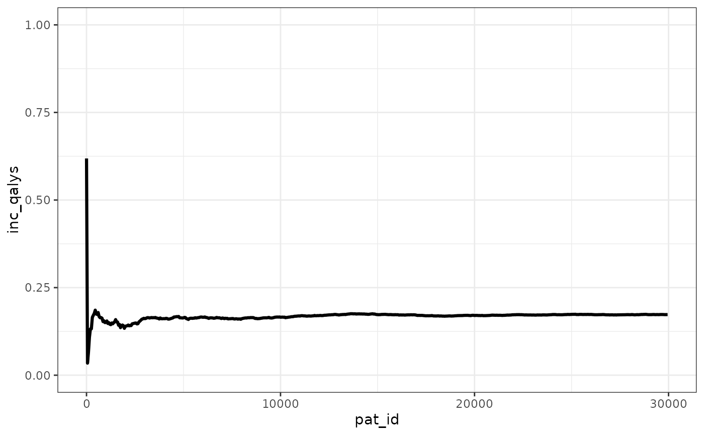
We can see that the ICER stabilizes pretty quickly, with the ICUR changing in absolute terms less than 500 GBP after 2,500 patients simulated.
merged_ipd <- psa_ipd  |>
  group_by(arm) |>
  mutate(cumul_total_qalys = cumsum(total_qalys)/pat_id,
         cumul_total_costs = cumsum(total_costs)/pat_id) |>
  transmute(pat_id, arm, cumul_total_qalys, cumul_total_costs) |>
  tidyr::pivot_wider(names_from = arm, values_from = c(cumul_total_qalys,cumul_total_costs)) |>
  mutate(inc_costs = cumul_total_costs_int - cumul_total_costs_comp,
         inc_qalys = cumul_total_qalys_int - cumul_total_qalys_comp,
         ICUR = inc_costs/ inc_qalys)

merged_ipd_results <- merged_ipd |> select(pat_id,inc_costs,inc_qalys,ICUR) |>  slice(seq(1, n(), by = 50))


ggplot(merged_ipd_results, aes(x=pat_id,y=ICUR))+
    geom_line(linewidth=1.1) +
    ylim(0,5000)+
    theme_bw() +
    theme(legend.position="bottom")
#> Warning: Removed 6 rows containing missing values or values outside the scale range
#> (`geom_line()`).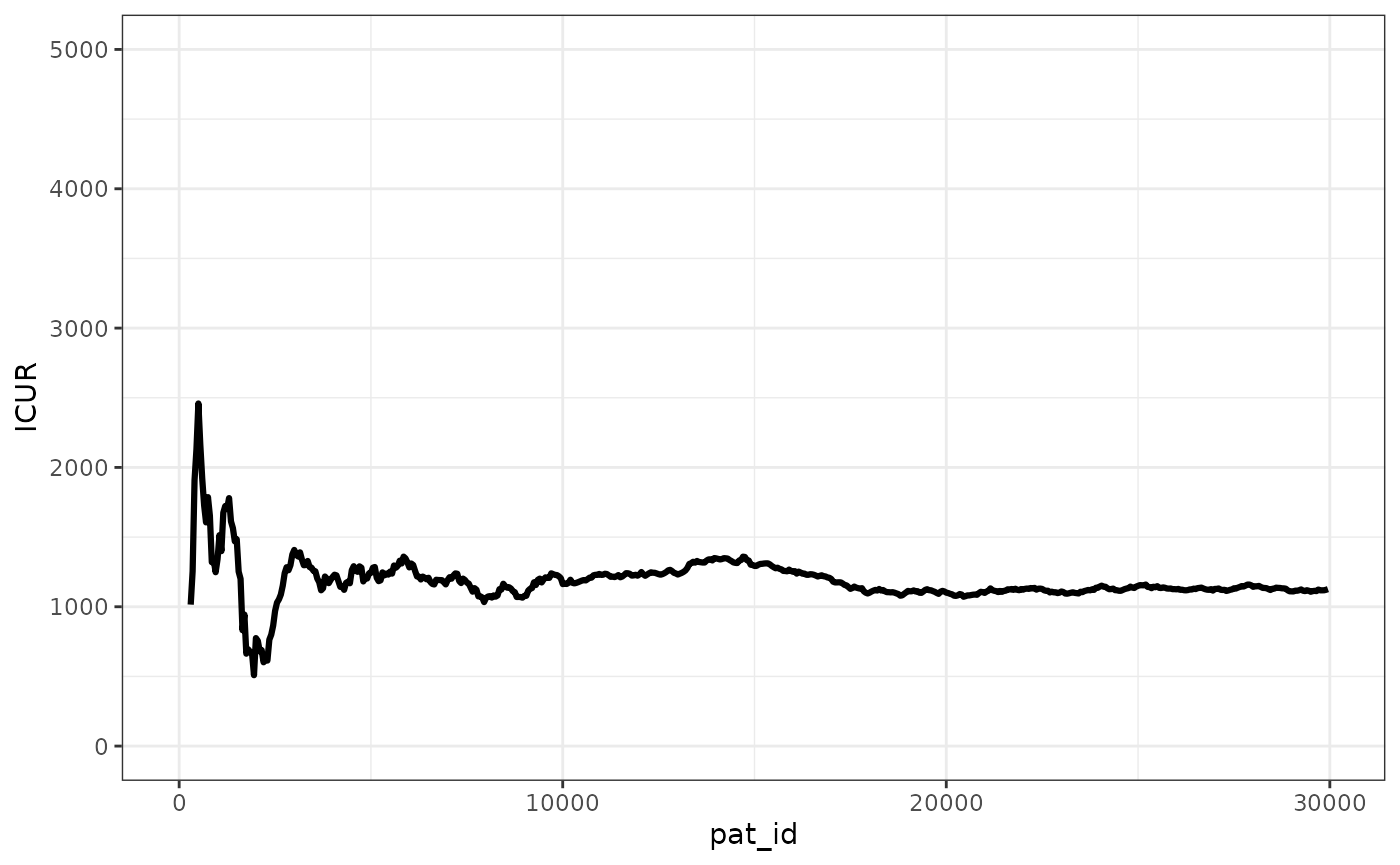
ggplot(merged_ipd_results, aes(x=pat_id,y=inc_costs))+
    geom_line(linewidth=1.1) +
    ylim(0,1000)+
    theme_bw() +
    theme(legend.position="bottom")
#> Warning: Removed 6 rows containing missing values or values outside the scale range
#> (`geom_line()`).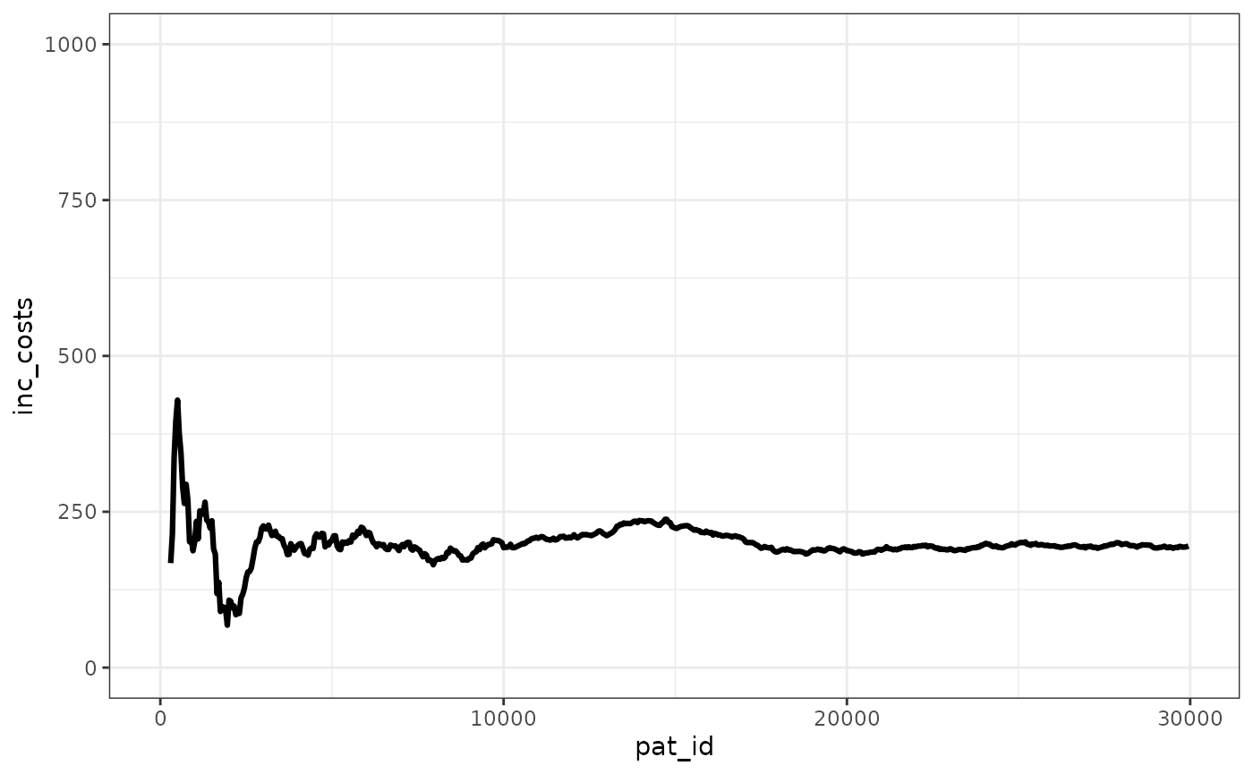
ggplot(merged_ipd_results, aes(x=pat_id,y=inc_qalys))+
    geom_line(linewidth=1.1) +
    ylim(0,1)+
    theme_bw() +
    theme(legend.position="bottom")